19.1. Sensing Matrices

19.1.1. Matrices Satisfying RIP

This section provides basic results about construction of matrices which can satisfy restricted isometry property.

The goal of designing an $M\times N$ sensing matrix involves:

• Stable embedding for signals with has high sparsity as possible (high $K$)

• As few measurements as possible (low $M$)

There are two different approaches

• Deterministic approach

• Randomized approach

Known deterministic approaches so far tend to require $M$ to be very large($O(K^2\ln N)$ or $O(K{N}^{\alpha }$). We can overcome this limitation by randomizing matrix construction.

Construction process:

• Input $M$ and $N$.

• Generate $\mathrm{\Phi }$ by choosing ${\mathrm{\Phi }}_{ij}$ as independent realizations from some probability distribution.

Suppose that $\mathrm{\Phi }$ is drawn from normal distribution.

It can be shown that the rank of $\mathrm{\Phi }$ is $M$ with probability $1$.

Example 19.1 (Random matrices are full rank.)

We can verify this fact by doing a small computer simulation.

M = 6;
N = 20;
trials = 10000;
numFullRankMatrices = 0;
for i=1:trials
    % Create a random matrix of size M x N
    A = rand(M,N);
    % Obtain its rank
    R = rank(A);
    % Check whether the rank equals M or not
    if R == M
        numFullRankMatrices = numFullRankMatrices + 1;
    end
end
fprintf('Number of trials: %d\n',trials);
fprintf('Number of full rank matrices: %d\n',numFullRankMatrices);
percentage = numFullRankMatrices*100/trials;
fprintf('Percentage of full rank matrices: %.2f %%\n', percentage);

This program generates a number of random matrices and measures their ranks. It verifies whether they are full rank or not.

Here is a sample output:

>> demoRandomMatrixRank
Number of trials: 10000
Number of full rank matrices: 10000
Percentage of full rank matrices: 100.00 

Thus if we choose $M=2K$, any subset of $2K$ columns will be linearly independent. Thus the matrix with satisfy RIP with some ${\delta }_{2K}>0$. But this construction doesn’t tell us exact value of ${\delta }_{2K}$. In order to find out ${\delta }_{2K}$, we must consider all possible $K$-dimensional subspaces of ${\mathbb{R}}^N$. This is computationally impossible for reasonably large $N$ and $K$. What is the alternative?

We can start with a chosen value of ${\delta }_{2K}$ and try to construct a matrix which matches it.

Before we proceed further, we should take a detour and review sub-Gaussian distributions in Subgaussian Distributions.

We now state the main theorem of this section.

Theorem 19.1 (Norm bounds on subgaussian vectors)

Suppose that $X=[X_1,X_2,\dots ,X_M]$ where each $X_i$ is i.i.d. with $X_i\sim \mathrm{Sub}(c^2)$ and $\mathbb{E}(X_i^2)={\sigma }^2$. Then

$$\mathbb{E}(\Vert X{\Vert }_2^2)=M{\sigma }^2$$

Moreover, for any $\alpha \in (0,1)$ and for any $\beta \in [c^2/{\sigma }^2,{\beta }_{\text{max}}$, there exists a constant ${\kappa }^{\ast }\ge 4$ depending only on ${\beta }_{\text{max}}$ and the ratio ${\sigma }^2/c^2$ such that

$$\mathbb{P}(\Vert X{\Vert }_2^2\le \alpha M{\sigma }^2)\le \exp (-\frac{M(1-\alpha {)}^2}{{\kappa }^{\ast }})$$

and

$$\mathbb{P}(\Vert X{\Vert }_2^2\ge \beta M{\sigma }^2)\le \exp (-\frac{M(\beta -1{)}^2}{{\kappa }^{\ast }})$$

19.1.1.1. Conditions on Random Distribution for RIP

Let us get back to our business of constructing a matrix $\mathrm{\Phi }$ using random distributions which satisfies RIP with a given $\delta$. We will impose some conditions on the random distribution.

• We require that the distribution will yield a matrix that is norm-preserving. This requires that

  (19.1)$$\mathbb{E}({\mathrm{\Phi }}_{ij}^2)=\frac{1}{M}$$

  Hence variance of distribution should be $\frac{1}{M}$.

• We require that distribution is a sub-Gaussian distribution; i.e., there exists a constant $c>0$ such that

  (19.2)$$\mathbb{E}(\exp ({\mathrm{\Phi }}_{ij}t))\le \exp \left(\frac{c^2{t}^2}{2}\right)$$

This says that the moment generating function of the distribution is dominated by a Gaussian distribution.
In other words, tails of the distribution decay at least as fast as the tails of a Gaussian distribution.

• We will further assume that entries of $\mathrm{\Phi }$ are strictly sub-Gaussian. i.e., they must satisfy (19.2) with

  $$c^2=\mathbb{E}({\mathrm{\Phi }}_{ij}^2)=\frac{1}{M}.$$

Under these conditions we have the following result.

Corollary 19.1 (Norm bounds on subgaussian matrix vector product)

Suppose that $\mathrm{\Phi }$ is an $M\times N$ matrix whose entries ${\mathrm{\Phi }}_{ij}$ are i.i.d. with ${\mathrm{\Phi }}_{ij}$ drawn according to a strictly sub-Gaussian distribution with $c^2=\frac{1}{M^2}$.

Let $Y=\mathrm{\Phi }x$ for $x\in {\mathbb{R}}^N$. Then for any $ϵ>0$ and any $x\in {\mathbb{R}}^N$,

$$\mathbb{E}(\Vert Y{\Vert }_2^2)=\Vert x{\Vert }_2^2$$

and

$$\mathbb{P}(\Vert Y{\Vert }_2^2-\Vert x{\Vert }_2^2\ge ϵ\Vert x{\Vert }_2^2)\le 2\exp (-\frac{M{ϵ}^2}{{\kappa }^{\ast }})$$

where ${\kappa }^{\ast }=\frac{2}{1-\ln (2)}\approx 6.5178$.

This means that the norm of a sub-Gaussian random vector strongly concentrates about its mean.

19.1.1.2. Sub Gaussian Matrices satisfy the RIP

Using this result we now state that sub-Gaussian matrices satisfy the RIP.

Theorem 19.2 (Lower bound on required number of measurements)

Fix $\delta \in (0,1)$. Let $\mathrm{\Phi }$ be an $M\times N$ random matrix whose entries ${\mathrm{\Phi }}_{ij}$ are i.i.d. with ${\mathrm{\Phi }}_{ij}$ drawn according to a strictly sub-Gaussian distribution with $c^2=\frac{1}{M}$. If

$$M\ge {\kappa }_{1}K\ln \left(\frac{N}{K}\right),$$

then $\mathrm{\Phi }$ satisfies the RIP of order $K$ with the prescribed $\delta$ with probability exceeding $1-2e^{-{\kappa }_{2}M}$, where ${\kappa }_1$ is arbitrary and

$${\kappa }_2=\frac{{\delta }^2}{2{\kappa }^{\ast }}-\frac{1}{{\kappa }_1}\ln \left(\frac{42e}{\delta }\right)$$

We note that this theorem achieves $M$ of the same order as the lower bound obtained in Theorem 18.42 up to a constant.

This is much better than deterministic approaches.

19.1.1.3. Advantages of Random Construction

There are a number of advantages of the random sensing matrix construction approach:

• One can show that for random construction, the measurements are democratic. This means that all measurements are equal in importance and it is possible to recover the signal from any sufficiently large subset of the measurements.

  Thus by using random $\mathrm{\Phi }$ one can be robust to the loss of loss or corruption of a small fraction of measurements.

• In general we are more interested in $x$ which is sparse in some basis $\mathrm{\Psi }$. In this setting, we require that $\mathrm{\Phi }\mathrm{\Psi }$ satisfy the RIP.

  Deterministic construction would explicitly require taking $\mathrm{\Psi }$ into account.

  But if $\mathrm{\Phi }$ is random, we can avoid this issue.

  If $\mathrm{\Phi }$ is Gaussian and $\mathrm{\Psi }$ is an orthonormal basis, then one can easily show that $\mathrm{\Phi }\mathrm{\Psi }$ will also have a Gaussian distribution.

  Thus if $M$ is high, $\mathrm{\Phi }\mathrm{\Psi }$ will also satisfy RIP with very high probability.

  Similar results hold for other sub-Gaussian distributions as well.

19.1.2. Rademacher Sensing Matrices

In this subsection, we collect several results related to Rademacher sensing matrices.

Definition 19.1

A Rademacher sensing matrix $\mathrm{\Phi }\in {\mathbb{R}}^{M\times N}$ with $M<N$ is constructed by drawing each entry ${\varphi }_{ij}$ independently from a Rademacher random distribution given by

(19.3)$${\mathbb{P}}_X(x)=\frac{1}{2}\delta (x-\frac{1}{\sqrt{M}})+\frac{1}{2}\delta (x+\frac{1}{\sqrt{M}}).$$

Thus ${\varphi }_{ij}$ takes a value $\pm \frac{1}{\sqrt{M}}$ with equal probability.

We can remove the scale factor $\frac{1}{\sqrt{M}}$ out of the matrix $\mathrm{\Phi }$ writing

$$\mathrm{\Phi }=\frac{1}{\sqrt{M}}\mathcal{X}$$

With that we can draw individual entries of $\mathcal{X}$ from a simpler Rademacher distribution given by

(19.4)$${\mathbb{P}}_X(x)=\frac{1}{2}\delta (x-1)+\frac{1}{2}\delta (x+1).$$

Thus entries in $\mathcal{X}$ take values of $\pm 1$ with equal probability.

This construction is useful since it allows us to implement the multiplication with $\mathrm{\Phi }$ in terms of just additions and subtractions. The scaling can be implemented towards the end in the signal processing chain.

We note that

$$\mathbb{E}({\varphi }_{ij})=0.$$

$$\mathbb{E}({\varphi }_{ij}^2)=\frac{1}{M}.$$

Actually we have a better result with

$${\varphi }_{ij}^2=\frac{1}{M}.$$

We can write

$$\mathrm{\Phi }=\left[\begin{array}{ccc}{\varphi }_1& \dots & {\varphi }_N\end{array}\right]$$

where ${\varphi }_j\in {\mathbb{R}}^M$ is a Rademacher random vector with independent entries. We note that

$$\mathbb{E}(\Vert {\varphi }_j{\Vert }_2^2)=\mathbb{E}\left(\sum _{i=1}^M{\varphi }_{ij}^2\right)=\sum _{i=1}^M(\mathbb{E}({\varphi }_{ij}^2))=M\frac{1}{M}=1.$$

In this case we also have

$$\Vert {\varphi }_j{\Vert }_2^2=1.$$

Thus the squared length of each of the columns in $\mathrm{\Phi }$ is $1$.

Lemma 19.1

Let $\mathbf{z}\in {\mathbb{R}}^M$ be a Rademacher random vector with i.i.d entries $z_i$ that take a value $\pm \frac{1}{\sqrt{M}}$ with equal probability. Let $\mathbf{u}\in {\mathbb{R}}^M$ be an arbitrary unit norm vector. Then

$$\mathbb{P}(|⟨\mathbf{z},\mathbf{u}⟩|>ϵ)\le 2\exp (-{ϵ}^2\frac{M}{2}).$$

Representative values of this bound are plotted below.

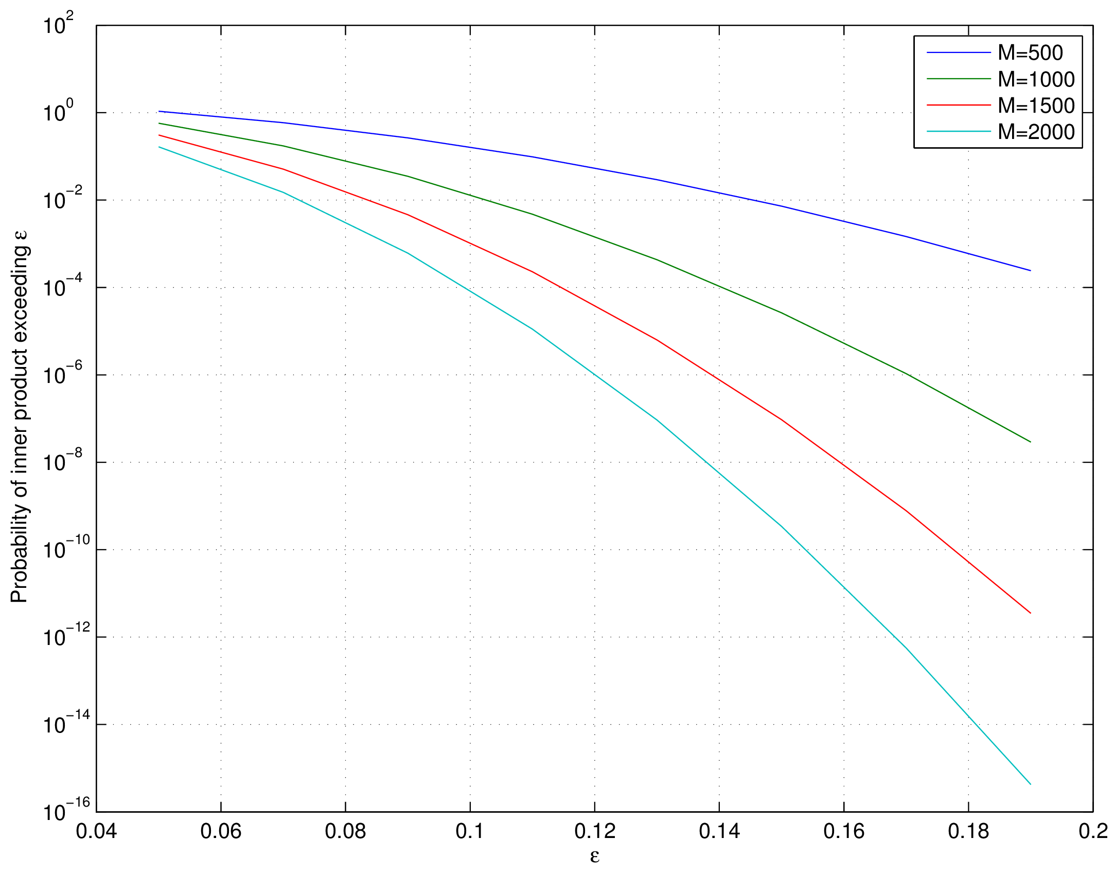
Fig. 19.1 Tail bound for the probability of inner product of a Rademacher random vector with a unit norm vector

Proof. This can be proven using Hoeffding’s inequality. To be elaborated later.

A particular application of this lemma is when $\mathbf{u}$ itself is another (independently chosen) unit norm Rademacher random vector.

The lemma establishes that the probability of inner product of two independent unit norm Rademacher random vectors being large is very very small. In other words, independently chosen unit norm Rademacher random vectors are incoherent with high probability. This is a very useful result as we will see later in measurement of coherence of Rademacher sensing matrices.

19.1.2.1. Joint Correlation

Columns of $\mathrm{\Phi }$ satisfy a joint correlation property ([80]) which is described in following lemma.

Lemma 19.2

Let $\{{\mathbf{u}}_k\}$ be a sequence of $K$ vectors (where ${\mathbf{u}}_k\in {\mathbb{R}}^M$) whose ${\ell }_2$ norms do not exceed one. Independently choose $\mathbf{z}\in {\mathbb{R}}^M$ to be a random vector with i.i.d. entries $z_i$ that take a value $\pm \frac{1}{\sqrt{M}}$ with equal probability. Then

$$\mathbb{P}(\underset{k}{max}|⟨\mathbf{z},{\mathbf{u}}_k⟩|\le ϵ)\ge 1-2K\exp (-{ϵ}^2\frac{M}{2}).$$

Proof. Let us call $\gamma =\underset{k}{max}|⟨\mathbf{z},{\mathbf{u}}_k⟩|$.

1. We note that if for any ${\mathbf{u}}_k$, $\Vert {\mathbf{u}}_k{\Vert }_2<1$ and we increase the length of ${\mathbf{u}}_k$ by scaling it, then $\gamma$ will not decrease and hence $\mathbb{P}(\gamma \le ϵ)$ will not increase.

2. Thus if we prove the bound for vectors ${\mathbf{u}}_k$ with $\Vert {\mathbf{u}}_k{\Vert }_2=1\mathrm{\forall }1\le k\le K$, it will be applicable for all ${\mathbf{u}}_k$ whose ${\ell }_2$ norms do not exceed one.

3. Hence we will assume that $\Vert {\mathbf{u}}_k{\Vert }_2=1$.

4. From Lemma 19.1 we have

   $$\mathbb{P}(|⟨z,u_k⟩|>ϵ)\le 2\exp (-{ϵ}^2\frac{M}{2}).$$

5. Now the event

   $$\{\underset{k}{max}|⟨z,u_k⟩|>ϵ\}=\bigcup _{k=1}^K\{|⟨z,u_k⟩|>ϵ\}$$

   i.e. if any of the inner products (absolute value) is greater than $ϵ$ then the maximum is greater.

6. We recall Boole’s inequality which states that

   $$\mathbb{P}\left(\bigcup _i{A}_i\right)\le \sum _i\mathbb{P}(A_i).$$

7. Thus

   $$\mathbb{P}(\underset{k}{max}|⟨\mathbf{z},{\mathbf{u}}_k⟩|>ϵ)\le 2K\exp (-{ϵ}^2\frac{M}{2}).$$

8. This gives us

   $$\begin{array}{rl}\mathbb{P}(\underset{k}{max}|⟨\mathbf{z},{\mathbf{u}}_k⟩|\le ϵ)& =1-\mathbb{P}(\underset{k}{max}|⟨\mathbf{z},{\mathbf{u}}_k⟩|>ϵ)\\ & \ge 1-2K\exp (-{ϵ}^2\frac{M}{2}).\end{array}$$

19.1.2.2. Coherence

We show that coherence of Rademacher sensing matrix is fairly small with high probability (adapted from [80]).

Lemma 19.3

Fix $\delta \in (0,1)$. For an $M\times N$ Rademacher sensing matrix $\mathrm{\Phi }$ as defined in Definition 19.1, the coherence statistic

$$\mu \le \sqrt{\frac{4}{M}\ln \left(\frac{N}{\delta }\right)}$$

with probability exceeding $1-\delta$.

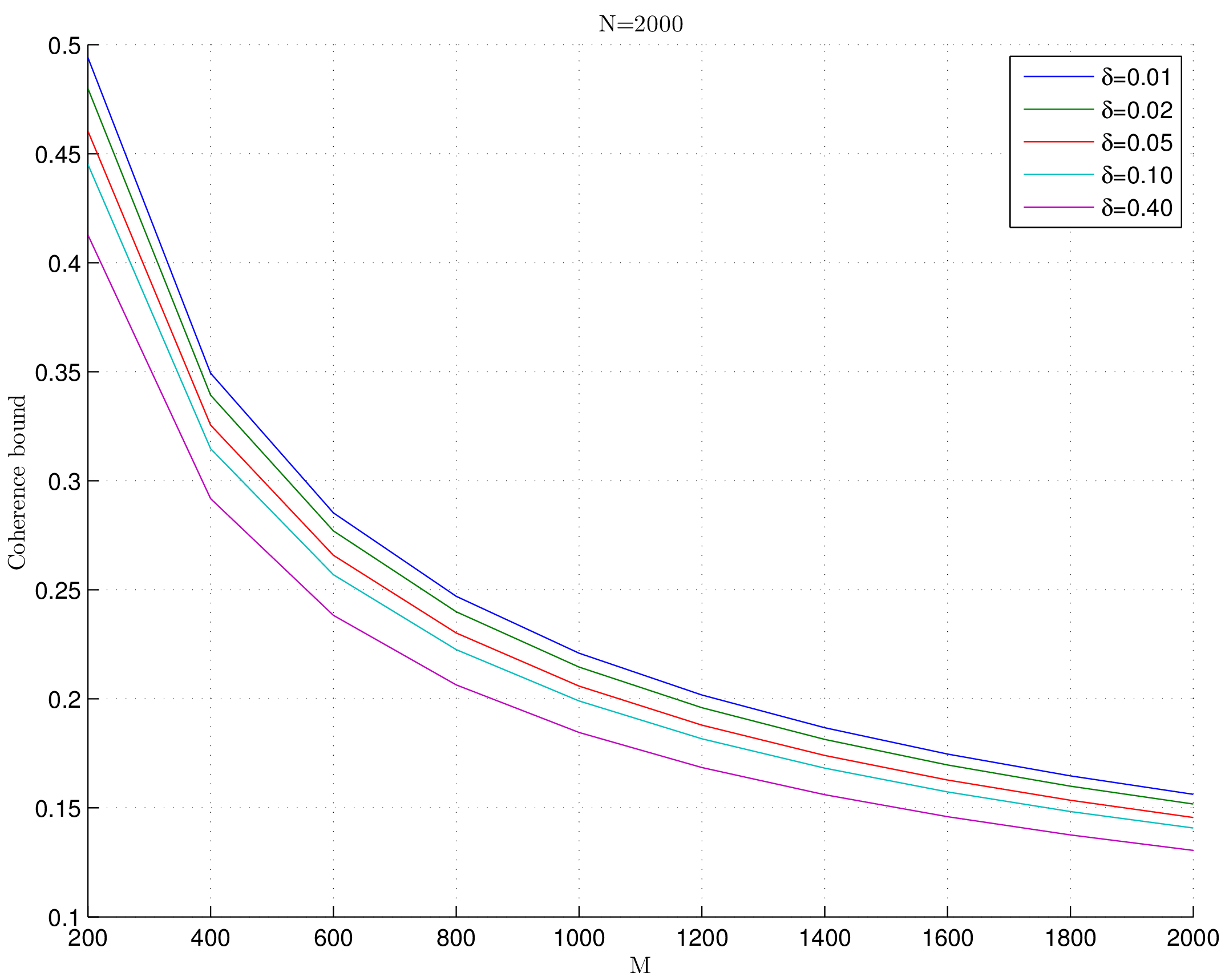
Fig. 19.2 Coherence bounds for Rademacher sensing matrices

Proof. We recall the definition of coherence as

$$\mu =\underset{j\ne k}{max}|⟨{\varphi }_j,{\varphi }_k⟩|=\underset{j<k}{max}|⟨{\varphi }_j,{\varphi }_k⟩|.$$

1. Since $\mathrm{\Phi }$ is a Rademacher sensing matrix hence each column of $\mathrm{\Phi }$ is unit norm column.

2. Consider some $1\le j<k\le N$ identifying columns ${\varphi }_j$ and ${\varphi }_k$.

3. We note that they are independent of each other.

4. Thus from Lemma 19.1 we have

   $$\mathbb{P}(|⟨{\varphi }_j,{\varphi }_k⟩|>ϵ)\le 2\exp (-{ϵ}^2\frac{M}{2}).$$

5. Now there are $\frac{N(N-1)}{2}$ such pairs of $(j,k)$.

6. Hence by applying Boole’s inequality

   $$\mathbb{P}(\underset{j<k}{max}|⟨{\varphi }_j,{\varphi }_k⟩|>ϵ)\le 2\frac{N(N-1)}{2}\exp (-{ϵ}^2\frac{M}{2})\le N^2\exp (-{ϵ}^2\frac{M}{2}).$$

7. Thus we have

   $$\mathbb{P}(\mu >ϵ)\le N^2\exp (-{ϵ}^2\frac{M}{2}).$$

8. What we need to do now is to choose a suitable value of $ϵ$ so that the R.H.S. of this inequality is simplified.

9. We choose

   $${ϵ}^2=\frac{4}{M}\ln \left(\frac{N}{\delta }\right).$$

10. This gives us

    $${ϵ}^2\frac{M}{2}=2\ln \left(\frac{N}{\delta }\right)⟹\exp (-{ϵ}^2\frac{M}{2})={\left(\frac{\delta }{N}\right)}^2.$$

11. Putting back we get

    $$\mathbb{P}(\mu >ϵ)\le N^2{\left(\frac{\delta }{N}\right)}^2\le {\delta }^2.$$

12. This justifies why we need $\delta \in (0,1)$.

13. Finally

    $$\mathbb{P}(\mu \le \sqrt{\frac{4}{M}\ln \left(\frac{N}{\delta }\right)})=\mathbb{P}(\mu \le ϵ)=1-\mathbb{P}(\mu >ϵ)>1-{\delta }^2$$

    and

    $$1-{\delta }^2>1-\delta$$

    which completes the proof.

19.1.3. Gaussian Sensing Matrices

In this subsection we collect several results related to Gaussian sensing matrices.

Definition 19.2

A Gaussian sensing matrix $\mathrm{\Phi }\in {\mathbb{R}}^{M\times N}$ with $M<N$ is constructed by drawing each entry ${\varphi }_{ij}$ independently from a Gaussian random distribution $\mathcal{N}(0,\frac{1}{M})$.

We note that

$$\mathbb{E}({\varphi }_{ij})=0.$$

$$\mathbb{E}({\varphi }_{ij}^2)=\frac{1}{M}.$$

We can write

$$\mathrm{\Phi }=\left[\begin{array}{ccc}{\varphi }_1& \dots & {\varphi }_N\end{array}\right]$$

where ${\varphi }_j\in {\mathbb{R}}^M$ is a Gaussian random vector with independent entries. We note that

$$\mathbb{E}(\Vert {\varphi }_j{\Vert }_2^2)=\mathbb{E}\left(\sum _{i=1}^M{\varphi }_{ij}^2\right)=\sum _{i=1}^M(\mathbb{E}({\varphi }_{ij}^2))=M\frac{1}{M}=1.$$

Thus the expected value of squared length of each of the columns in $\mathrm{\Phi }$ is $1$.

19.1.3.1. Joint Correlation

Columns of $\mathrm{\Phi }$ satisfy a joint correlation property ([80]) which is described in following lemma.

Lemma 19.4

Let $\{{\mathbf{u}}_k\}$ be a sequence of $K$ vectors (where ${\mathbf{u}}_k\in {\mathbb{R}}^M$) whose ${\ell }_2$ norms do not exceed one. Independently choose $\mathbf{z}\in {\mathbb{R}}^M$ to be a random vector with i.i.d. $\mathcal{N}(0,\frac{1}{M})$ entries. Then

$$\mathbb{P}(\underset{k}{max}|⟨z,u_k⟩|\le ϵ)\ge 1-K\exp (-{ϵ}^2\frac{M}{2}).$$

Proof. Let us call $\gamma =\underset{k}{max}|⟨\mathbf{z},{\mathbf{u}}_k⟩|$.

1. We note that if for any ${\mathbf{u}}_k$, $\Vert {\mathbf{u}}_k{\Vert }_2<1$ and we increase the length of ${\mathbf{u}}_k$ by scaling it, then $\gamma$ will not decrease and hence $\mathbb{P}(\gamma \le ϵ)$ will not increase.

2. Thus if we prove the bound for vectors ${\mathbf{u}}_k$ with $\Vert {\mathbf{u}}_k{\Vert }_2=1\mathrm{\forall }1\le k\le K$, it will be applicable for all ${\mathbf{u}}_k$ whose ${\ell }_2$ norms do not exceed one.

3. Hence we will assume that $\Vert {\mathbf{u}}_k{\Vert }_2=1$.

4. Now consider $⟨\mathbf{z},{\mathbf{u}}_k⟩$.

5. Since $\mathbf{z}$ is a Gaussian random vector, hence $⟨\mathbf{z},{\mathbf{u}}_k⟩$ is a Gaussian random variable.

6. Since $\Vert {\mathbf{u}}_k\Vert =1$ hence

   $$⟨\mathbf{z},{\mathbf{u}}_k⟩\sim \mathcal{N}(0,\frac{1}{M}).$$

7. We recall a well known tail bound for Gaussian random variables which states that

   $${\mathbb{P}}_X(|x|>ϵ)=\sqrt{\frac{2}{\pi }}{\int }_{ϵ\sqrt{N}}^{\mathrm{\infty }}\exp (-\frac{x^2}{2})dx\le \exp (-{ϵ}^2\frac{M}{2}).$$

8. Now the event

   $$\{\underset{k}{max}|⟨\mathbf{z},{\mathbf{u}}_k⟩|>ϵ\}=\bigcup _{k=1}^K\{|⟨\mathbf{z},{\mathbf{u}}_k⟩|>ϵ\}$$

   i.e. if any of the inner products (absolute value) is greater than $ϵ$ then the maximum is greater.

9. We recall Boole’s inequality which states that

   $$\mathbb{P}\left(\bigcup _i{A}_i\right)\le \sum _i\mathbb{P}(A_i).$$

10. Thus

    $$\mathbb{P}(\underset{k}{max}|⟨\mathbf{z},{\mathbf{u}}_k⟩|>ϵ)\le K\exp (-{ϵ}^2\frac{M}{2}).$$

11. This gives us

    $$\begin{array}{r}\begin{array}{rl}\mathbb{P}(\underset{k}{max}|⟨\mathbf{z},{\mathbf{u}}_k⟩|\le ϵ)& =1-\mathbb{P}(\underset{k}{max}|⟨\mathbf{z},{\mathbf{u}}_k⟩|>ϵ)\\ & \ge 1-K\exp (-{ϵ}^2\frac{M}{2}).\end{array}\end{array}$$