23. Subspace Clustering

High dimensional data-sets are now pervasive in various signal processing applications. For example, high resolution surveillance cameras are now commonplace generating millions of images continually. A major factor in the success of current generation signal processing algorithms is the fact that, even though these data-sets are high dimensional, their intrinsic dimension is often much smaller than the dimension of the ambient space.

One resorts to inferring (or learning) a quantitative model $\mathbb{M}$ of a given set of data points $\mathbf{Y}=\{{\mathbf{y}}_1,\dots ,{\mathbf{y}}_S\}\subset {\mathbb{R}}^M$. Such a model enables us to obtain a low dimensional representation of a high dimensional data set. The low dimensional representations enable efficient implementation of acquisition, compression, storage, and various statistical inferencing tasks without losing significant precision. There is no such thing as a perfect model. Rather, we seek a model ${\mathbb{M}}^{\ast }$ that is best among a restricted class of models $\mathcal{M}=\{\mathbb{M}\}$ which is rich enough to describe the data set to a desired accuracy yet restricted enough so that selecting the best model is tractable.

In absence of training data, the problem of modeling falls into the category of unsupervised learning. There are two common viewpoints of data modeling. A statistical viewpoint assumes that data points are random samples from a probabilistic distribution. Statistical models try to learn the distribution from the dataset. In contrast, a geometrical viewpoint assumes that data points belong to a geometrical object (a smooth manifold or a topological space). A geometrical model attempts to learn the shape of the object to which the data points belong. Examples of statistical modeling include maximum likelihood, maximum a posteriori estimates, Bayesian models etc. An example of geometrical models is Principal Component Analysis (PCA) which assumes that data is drawn from a low dimensional subspace of the high dimensional ambient space. PCA is simple to implement and has found tremendous success in different fields e.g., pattern recognition, data compression, image processing, computer vision, etc. 1.

The assumption that all the data points in a data set could be drawn from a single model however happens to be a stretched one. In practice, it often occurs that if we group or segment the data set $\mathbf{Y}$ into multiple disjoint subsets: $\mathbf{Y}={\mathbf{Y}}_1\cup \cdots \cup {\mathbf{Y}}_K$, then each subset can be modeled sufficiently well by a model ${\mathbb{M}}_k^{\ast }$ ($1\le k\le K$) chosen from a simple model class. Each model ${\mathbb{M}}_k^{\ast }$ is called a primitive or component model. In this sense, the data set $\mathbf{Y}$ is called a mixed dataset and the collection of primitive models is called a hybrid model for the dataset. Let us look at some examples of mixed data sets.

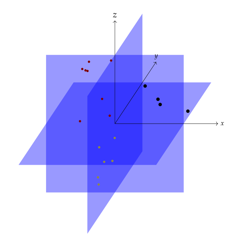
Consider the problem of vanishing point detection in computer vision. Under perspective projection, a group of parallel lines pass through a common point in the image plane which is known as the vanishing point for the group. For a typical scene consisting of multiple sets of parallel lines, the problem of detecting all vanishing points in the image plane from the set of edge segments (identified in the image) can be transformed into clustering points (in edge segments) into multiple 2D subspaces in ${\mathbb{R}}^3$ (world coordinates of the scene).

In the Motion segmentation problem, an image sequence consisting of multiple moving objects is segmented so that each segment consists of motion from only one object. This is a fundamental problem in applications such as motion capture, vision based navigation, target tracking and surveillance. We first track the trajectories of feature points (from all objects) over the image sequence. It has been shown (see sec:motion_segmentation) that trajectories of feature points for rigid motion for a single object form a low dimensional subspace. Thus motion segmentation problem can be solved by segmenting the feature point trajectories
for different objects separately and estimating the motion of each object from corresponding trajectories.

In a face clustering problem, we have a collection of unlabeled images of different faces taken under varying illumination conditions. Our goal is to cluster, images of the same face in one group each. For a Lambertian object, it has been shown that the set of images taken under different lighting conditions forms a cone in the image space. This cone can be well approximated by a low-dimensional subspace [5, 49]. The images of the face of each person form one low dimensional subspace and the face clustering problem reduces to clustering the collection of images to multiple subspaces.

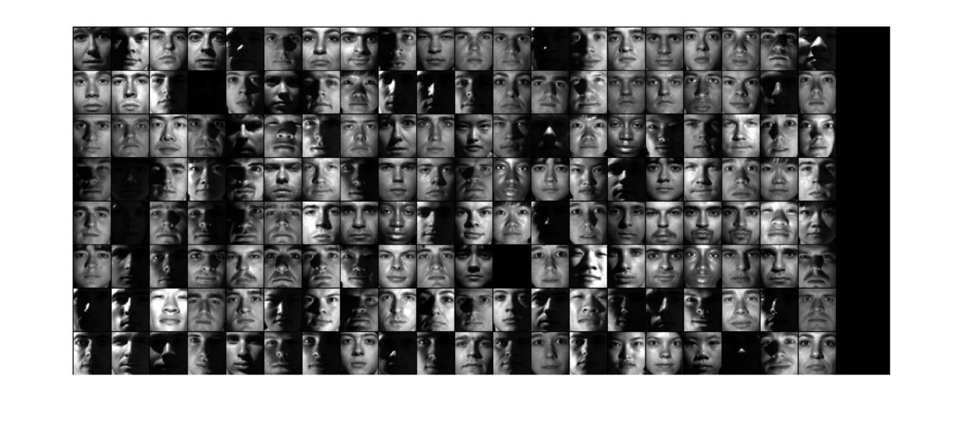
Fig. 23.1 A sample of faces from the Extended Yale Faces dataset B [40]. It contains 16128 images of 28 human subjects under 9 poses and 64 illumination conditions.

As the examples above suggest, a typical hybrid model for a mixed data set consists of multiple primitive models where each primitive is a (low dimensional) subspace. The data set is modeled as being sampled from a collection or arrangement $\mathcal{U}$ of linear (or affine) subspaces ${\mathcal{U}}_k\subset {\mathbb{R}}^M$ : $\mathcal{U}=\{{\mathcal{U}}_1,\dots ,{\mathcal{U}}_K\}$. The union of the subspaces2 is denoted as $Z_{\mathcal{U}}={\mathcal{U}}_1\cup \cdots \cup {\mathcal{U}}_K$. This is indeed a geometric model. In such modeling problems, individual subspaces (dimension and orientation of each subspace and total number of subspaces) and the membership of a data point (a single image in the face clustering problem) to a particular subspace is unknown beforehand. This entails the need for algorithms which can simultaneously identify the subspaces involved and cluster/segment the data points from individual subspaces into separate groups. This problem is known as subspace clustering which is the focus of this paper. An earlier detailed introduction to subspace clustering can be found in [83].

An example of a statistical hybrid model is a Gaussian Mixture Model (GMM) where one assumes that the sample points are drawn independently from a mixture of Gaussian distributions. A way of estimating such a mixture model is the expectation maximization (EM) method.

The fundamental difficulty in the estimation of hybrid models is the “chicken-and-egg” relationship between data segmentation and model estimation. If the data segmentation was known, one could easily fit a primitive model to each subset. Alternatively, if the constituent primitive models were known, one could easily segment the data by choosing the best model for each data point. An iterative approach starts with an initial (hopefully good) guess of primitive models or data segments. It then alternates between estimating the models for each segment and segmenting the data based on current primitive models till the solution converges. On the contrary, a global algorithm can perform the segmentation and primitive modeling simultaneously. In the sequel, we will look at a variety of algorithms for solving the subspace clustering problem.

23.1. Notation

First some general notation for vectors and matrices.

1. For a vector $\mathbf{v}\in {\mathbb{R}}^n$, its support is denoted by $\mathrm{supp}(\mathbf{v})$ and is defined as $\mathrm{supp}(\mathbf{v})\triangleq \{i:v_i\ne 0,1\le i\le n\}$.

2. $|\mathbf{v}|$ denotes a vector obtained by taking the absolute values of entries in $\mathbf{v}$.

3. ${\mathbf{1}}_n\in {\mathbb{R}}^n$ denotes a vector whose every entry is $1$.

4. $\Vert \mathbf{v}{\Vert }_p$ denotes the ${\ell }_p$ norm of $v$.

5. $\Vert \mathbf{v}{\Vert }_0$ denotes the ${\ell }_0$-“norm” of $\mathbf{v}$.

6. Let $\mathbf{A}$ be any $m\times n$ real matrix ($\mathbf{A}\in {\mathbb{R}}^{m\times n}$).

7. $a_{i,j}$ is the element at the $i$-th row and $j$-th column of $\mathbf{A}$.

8. ${\mathbf{a}}_j$ with $1\le j\le n$ denotes the $j$-th column vector of $\mathbf{A}$.

9. ${\underset{―}{a}}_i$ with $1\le i\le m$ denotes the $i$-th row vector of $\mathbf{A}$.

10. $a_{j,k}$ is the $k$-th entry in ${\mathbf{a}}_j$.

11. ${\underset{―}{a}}_{i,k}$ is the $k$-th entry in ${\underset{―}{a}}_i$.

12. ${\mathbf{A}}_{\mathrm{\Lambda }}$ denotes a submatrix of $\mathbf{A}$ consisting of columns indexed by $\mathrm{\Lambda }\subset \{1,\dots ,n\}$.

13. ${\underset{―}{\mathbf{A}}}_{\mathrm{\Lambda }}$ denotes a submatrix of $\mathbf{A}$ consisting of rows indexed by $\mathrm{\Lambda }\subset \{1,\dots ,m\}$.

14. $|\mathbf{A}|$ denotes the matrix consisting of absolute values of entries in $\mathbf{A}$.

15. $\mathrm{supp}(\mathbf{A})$ denotes the index set of non-zero rows of $\mathbf{A}$.

16. Clearly, $\mathrm{supp}(\mathbf{A})\subseteq \{1,\dots ,m\}$.

17. $\Vert \mathbf{A}{\Vert }_0$ denotes the number of non-zero rows of $\mathbf{A}$.

18. Clearly, $\Vert \mathbf{A}{\Vert }_0=|\mathrm{supp}(\mathbf{A})|$.

19. We note that while $\Vert \mathbf{A}{\Vert }_0$ is not a norm, its behavior is similar to the ${\ell }_0$-“norm” for vectors $\mathbf{v}\in {\mathbb{R}}^n$ defined as $\Vert \mathbf{v}{\Vert }_0\triangleq |\mathrm{supp}(\mathbf{v})|$.

20. We use $f(x)$ and $F(x)$ to denote the PDF and CDF of a continuous random variable.

21. We use $p(x)$ to denote the PMF of a discrete random variable.

22. We use $\mathbb{P}(E)$ to denote the probability of an event.

23.1.1. Problem Formulation

The data set can be modeled as a set of data points lying in a union of low dimensional linear or affine subspaces in a Euclidean space ${\mathbb{R}}^M$ where $M$ denotes the dimension of ambient space.

1. Let the data set be $\{{\mathbf{y}}_j\in {\mathbb{R}}^M{\}}_{j=1}^S$ drawn from the union of subspaces under consideration.

2. $S$ is the total number of data points being analyzed simultaneously.

3. We put the data points together in a data matrix as

   $$\mathbf{Y}\triangleq \left[\begin{array}{ccc}{\mathbf{y}}_1& \dots & {\mathbf{y}}_S\end{array}\right].$$

4. The data matrix $Y$ is known to us.

5. Note that in statistic books, data samples are placed in each row of the data matrix. We are putting data samples in each column of the data matrix.

6. We will slightly abuse the notation and let $\mathbf{Y}$ denote the set of data points $\{{\mathbf{y}}_j\in {\mathbb{R}}^M{\}}_{j=1}^S$ also.

7. We will use the terms data points and vectors interchangeably.

8. Let the vectors be drawn from a set of $K$ (linear or affine) subspaces.

9. The number of subspaces may not be known in advance.

10. The subspaces are indexed by a variable $k$ with $1\le k\le K$.

11. The $k$-th subspace is denoted by ${\mathcal{U}}_k$.

12. Let the (linear or affine) dimension of $k$-th subspace be $\dim ({\mathcal{U}}_k)=D_k$ with $D_k\le D$.

13. Here $D$ is an upper bound on the dimension of individual subspaces.

14. We may or may not know $D$.

15. We assume that none of the subspaces is contained in another.

16. A pair of subspaces may not intersect (e.g. parallel lines or planes), may have a trivial intersection (lines passing through origin), or a non-trivial intersection (two planes intersecting at a line).

17. The collection of subspaces may also be independent or disjoint (see Linear Algebra).

18. The vectors in $\mathbf{Y}$ can be grouped (or segmented or clustered) as submatrices ${\mathbf{Y}}_1,{\mathbf{Y}}_2,\dots ,{\mathbf{Y}}_K$ such that all vectors in ${\mathbf{Y}}_k$ lie in subspace ${\mathcal{U}}_k$.

19. Thus, we can write

    $${\mathbf{Y}}^{\ast }=\mathbf{Y}\mathrm{\Gamma }=\left[\begin{array}{ccc}{\mathbf{y}}_1& \dots & {\mathbf{y}}_S\end{array}\right]\mathrm{\Gamma }=\left[\begin{array}{ccc}{\mathbf{Y}}_1& \dots & {\mathbf{Y}}_K\end{array}\right]$$

    where $\mathrm{\Gamma }$ is an $S\times S$ unknown permutation matrix placing each vector to the right subspace.

20. This segmentation is straight-forward if the (affine) subspaces do not intersect or the subspaces intersect trivially at one point (e.g. any pair of linear subspaces passes through origin).

21. Let there be $S_k$ vectors in ${\mathbf{Y}}_k$ with $S=S_1+\cdots +S_K$.

22. We may not have any prior information about the number of points in individual subspaces.

23. We do typically require that there are enough vectors drawn from each subspace so that they can span the corresponding subspace.

24. This requirement may vary for individual subspace clustering algorithms.

25. For example, for linear subspaces, sparse representation based algorithms require that whenever a vector is removed from ${\mathbf{Y}}_k$, the remaining set of vectors spans ${\mathcal{U}}_k$.

26. This guarantees that every vector in ${\mathbf{Y}}_k$ can be represented in terms of other vectors in ${\mathbf{Y}}_k$.

27. The minimum required $S_k$ for which this is possible is $S_k=D_k+1$ when the data points from each subspace are in general position (i.e. $\mathrm{spark}({\mathbf{Y}}_k)=D_k+1$).

28. Let ${\mathbf{Q}}_k$ be an orthonormal basis for subspace ${\mathcal{U}}_k$.

29. Then, the subspaces can be described as

    $${\mathcal{U}}_k=\{\mathbf{y}\in {\mathbb{R}}^M|\mathbf{y}={\mu }_k+{\mathbf{Q}}_k\mathbf{a}\},1\le k\le K$$

30. For linear subspaces, ${\mu }_k=\mathbf{0}$.

31. We will abuse ${\mathbf{Y}}_k$ to also denote the set of vectors from the $k$-th subspace.

32. The basic objective of subspace clustering algorithms is to obtain a clustering or segmentation of vectors in $\mathbf{Y}$ into ${\mathbf{Y}}_1,\dots ,{\mathbf{Y}}_K$.

33. This involves finding out the number of subspaces/clusters $K$, and placing each vector ${\mathbf{y}}_s$ in its cluster correctly.

34. Alternatively, if we can identify $\mathrm{\Gamma }$ and the numbers $S_1,\dots ,S_K$ correctly, we have solved the clustering problem.

35. Since the clusters fall into different subspaces, as part of subspace clustering, we may also identify the dimensions $\{D_k{\}}_{k=1}^K$ of individual subspaces, the bases $\{{\mathbf{Q}}_k{\}}_{k=1}^K$ and the offset vectors $\{{\mu }_k{\}}_{k=1}^K$ in case of affine subspaces.

36. These quantities emerge due to modeling the clustering problem as a subspace clustering problem.

37. However, they are not essential outputs of the subspace clustering algorithms.

38. Some subspace clustering algorithms may not calculate them, yet they are useful in the analysis of the algorithm.

39. See Data Clustering for a quick review of data clustering terminology.

23.1.2. Noisy Case

1. We also consider clustering of data points which are contaminated with noise.

2. The data points do not perfectly lie in a subspace but can be approximated as a sum of a component which lies perfectly in a subspace and a noise component.

3. Let

   $${\mathbf{y}}_s={\overline{\mathbf{y}}}_s+{\mathbf{e}}_s,\mathrm{\forall }1\le s\le S$$

   be the $s$-th vector that is obtained by corrupting an error free vector ${\overline{\mathbf{y}}}_s$ (which perfectly lies in a low dimensional subspace) with a noise vector ${\mathbf{e}}_s\in {\mathbb{R}}^M$.

4. The clustering problem remains the same. Our goal would be to characterize the behavior of the clustering algorithm in the presence of noise at different levels.

23.2. Linear Algebra

This section reviews some useful concepts from linear algebra relevant for the chapter.

A collection of linear subspaces $\{{\mathcal{U}}^i{\}}_{i=1}^n$ is called independent if $\dim ({\oplus }_{i=1}^n{\mathcal{U}}^i)$ equals $\sum _{i=1}^n\dim ({\mathcal{U}}^i)$.

A collection of linear subspaces is called disjoint if they are pairwise independent [33]. In other words, every pair of subspaces intersect only at the origin.

23.2.1. Affine Subspaces

For a detailed introduction to affine concepts, see [54].

1. For a vector $\mathbf{v}\in {\mathbb{R}}^n$, the function $f$ defined by $f(\mathbf{x})=\mathbf{x}+\mathbf{v},\mathbf{x}\in {\mathbb{R}}^n$ is a translation of ${\mathbb{R}}^n$ by $\mathbf{v}$.

2. The image of any set $\mathcal{S}$ under $f$ is the $\mathbf{v}$-translate of $\mathcal{S}$.

3. A translation of space is a one to one isometry of ${\mathbb{R}}^n$ onto ${\mathbb{R}}^n$.

4. A translate of a $d$-dimensional linear subspace of ${\mathbb{R}}^n$ is a $d$-dimensional flat or simply $d$-flat in ${\mathbb{R}}^n$.

5. Flats of dimension 1, 2, and $n-1$ are also called lines, planes, and hyperplanes, respectively.

6. Flats are also known as affine subspaces.

7. Every $d$-flat in ${\mathbb{R}}^n$ is congruent to the Euclidean space ${\mathbb{R}}^d$.

8. Flats are closed sets.

Affine combinations

1. An affine combination of the vectors ${\mathbf{v}}_1,\dots ,{\mathbf{v}}_m$ is a linear combination in which the sum of coefficients is 1.

2. Thus, $\mathbf{b}$ is an affine combination of ${\mathbf{v}}_1,\dots ,{\mathbf{v}}_m$ if $\mathbf{b}=k_1{\mathbf{v}}_1+\dots k_m{\mathbf{v}}_m$ and $k_1+\cdots +k_m=1$.

3. The set of affine combinations of a set of vectors $\{{\mathbf{v}}_1,\dots ,{\mathbf{v}}_m\}$ is their affine span.

4. A finite set of vectors $\{{\mathbf{v}}_1,\dots ,{\mathbf{v}}_m\}$ is called affine independent if the only zero-sum linear combination representing the null vector is the null combination. i.e. $k_1{\mathbf{v}}_1+\cdots +k_m{\mathbf{v}}_m=\mathbf{0}$ and $k_1+\cdots +k_m=0$ implies $k_1=\cdots =k_m=0$.

5. Otherwise, the set is affinely dependent.

6. A finite set of two or more vectors is affine independent if and only if none of them is an affine combination of the others.

Vectors vs. Points

1. We often use capital letters to denote points and bold small letters to denote vectors.

2. The origin is referred to by the letter $O$.

3. An n-tuple $(x_1,\dots ,x_n)$ is used to refer to a point $X$ in ${\mathbb{R}}^n$ as well as to a vector from origin $O$ to $X$ in ${\mathbb{R}}^n$.

4. In basic linear algebra, the terms vector and point are used interchangeably.

5. While discussing geometrical concepts (affine or convex sets etc.), it is useful to distinguish between vectors and points.

6. When the terms “dependent” and “independent” are used without qualification to points, they refer to affine dependence/independence.

7. When used for vectors, they mean linear dependence/independence.

$k$-flats

1. The span of $k+1$ independent points is a $k$-flat and is the unique $k$-flat that contains all $k+1$ points.

2. Every $k$-flat contains $k+1$ (affine) independent points.

3. Each set of $k+1$ independent points in the $k$-flat forms an affine basis for the flat.

4. Each point of a $k$-flat is represented by one and only one affine combination of a given affine basis for the flat.

5. The coefficients of the affine combination of a point are the affine coordinates of the point in the given affine basis of the $k$-flat.

6. A $d$-flat is contained in a linear subspace of dimension $d+1$.

7. This can be easily obtained by choosing an affine basis for the flat and constructing its linear span.

Affine functions

1. A function $f$ defined on a vector space $\mathbb{V}$ is an affine function or affine transformation or affine mapping if it maps every affine combination of vectors $\mathbf{u},\mathbf{v}$ in $\mathbb{V}$ onto the same affine combination of their images.

2. If $f$ is real valued, then $f$ is an affine functional.

3. A property which is invariant under an affine mapping is called affine invariant.

4. The image of a flat under an affine function is a flat.

5. Every affine function differs from a linear function by a translation.

Affine functionals

1. A functional is an affine functional if and only if there exists a unique vector $\mathbf{a}\in {\mathbb{R}}^n$ and a unique real number $k$ such that $f(\mathbf{x})=⟨\mathbf{a},\mathbf{x}⟩+k$.

2. Affine functionals are continuous.

3. If $\mathbf{a}\ne \mathbf{0}$, then the linear functional $f(\mathbf{x})=⟨\mathbf{a},\mathbf{x}⟩$ and the affine functional $g(\mathbf{x})=⟨\mathbf{a},\mathbf{x}⟩+k$ map bounded sets onto bounded sets, neighborhoods onto neighborhoods, balls onto balls and open sets onto open sets.

23.2.2. Hyperplanes and Halfspaces

1. Corresponding to a hyperplane $\mathcal{H}$ in ${\mathbb{R}}^n$ (an $n-1$-flat), there exists a non-null vector $\mathbf{a}$ and a real number $k$ such that $\mathcal{H}$ is the graph of $⟨\mathbf{a},\mathbf{x}⟩=k$.

2. The vector $\mathbf{a}$ is orthogonal to $PQ$ for all $P,Q\in \mathcal{H}$.

3. All non-null vectors $\mathbf{a}$ to have this property are normal to the hyperplane.

4. The directions of $\mathbf{a}$ and $-\mathbf{a}$ are called opposite normal directions of $\mathcal{H}$.

5. Conversely, the graph of $⟨\mathbf{a},\mathbf{x}⟩=k$, $\mathbf{a}\ne \mathbf{0}$, is a hyperplane for which $\mathbf{a}$ is a normal vector. If $⟨a,x⟩=k$ and $⟨\mathbf{b},\mathbf{x}⟩=h$, $\mathbf{a}\ne \mathbf{0}$, $\mathbf{b}\ne \mathbf{0}$ are both representations of a hyperplane $\mathcal{H}$, then there exists a real non-zero number $\lambda$ such that $\mathbf{b}=\lambda \mathbf{a}$ and $h=\lambda k$.

6. We can find a unit norm normal vector for $\mathcal{H}$.

7. Each point $P$ in space has a unique foot (nearest point) $P_0$ in a Hyperplane $\mathcal{H}$.

8. Distance of the point $P$ with vector $\mathbf{p}$ from a hyperplane $\mathcal{H}:⟨\mathbf{a},\mathbf{x}⟩=k$ is given by

   $$d(P,\mathcal{H})=\frac{|⟨\mathbf{a},\mathbf{p}⟩-k|}{\Vert \mathbf{a}{\Vert }_2}.$$

9. The coordinate ${\mathbf{p}}_0$ of the foot $P_0$ is given by

   $${\mathbf{p}}_0=\mathbf{p}-\frac{⟨\mathbf{a},\mathbf{p}⟩-k}{\Vert \mathbf{a}{\Vert }_2^2}\mathbf{a}.$$

10. Hyperplanes $\mathcal{H}$ and $\mathcal{K}$ are parallel if they don’t intersect.

11. This occurs if and only if they have a common normal direction.

12. They are different constant sets of the same linear functional.

13. If ${\mathcal{H}}_1:⟨\mathbf{a},\mathbf{x}⟩=k_1$ and ${\mathcal{H}}_2:⟨\mathbf{a},\mathbf{x}⟩=k_2$ are parallel hyperplanes, then the distance between the two hyperplanes is given by

    $$d({\mathcal{H}}_1,{\mathcal{H}}_2)=\frac{|k_1-k_2|}{\Vert \mathbf{a}{\Vert }_2}.$$

Half-spaces

1. If $⟨\mathbf{a},\mathbf{x}⟩=k$, $\mathbf{a}\ne \mathbf{0}$, is a hyperplane $\mathcal{H}$, then the graphs of $⟨\mathbf{a},\mathbf{x}⟩>k$ and $⟨\mathbf{a},\mathbf{x}⟩<k$ are the opposite sides or opposite open half spaces of $\mathcal{H}$.

2. The graphs of $⟨\mathbf{a},\mathbf{x}⟩\ge k$ and $⟨\mathbf{a},\mathbf{x}⟩\le k$ are the opposite closed half spaces of $\mathcal{H}$.

3. $\mathcal{H}$ is the face of the four half-spaces.

4. Corresponding to a hyperplane $\mathcal{H}$, there exists a unique pair of sets ${\mathcal{S}}_1$ and ${\mathcal{S}}_2$ that are the opposite sides of $\mathcal{H}$.

5. Open half spaces are open sets and closed half spaces are closed sets.

6. If $A$ and $B$ belong to the opposite sides of a hyperplane $\mathcal{H}$, then there exists a unique point of $\mathcal{H}$ that is between $A$ and $B$.

23.2.3. General Position

1. A general position for a set of points or other geometric objects is a notion of genericity.

2. It means the general case situation as opposed to more special and coincidental cases.

3. For example, generically, two lines in a plane intersect in a single point.

4. The special cases are when the two lines are either parallel or coincident.

5. Three points in a plane in general are not collinear.

6. If they are, then it is a degenerate case.

7. A set of $n+1$ or more points in ${\mathbb{R}}^n$ is in said to be in general position if every subset of $n$ points is linearly independent.

8. In general, a set of $k+1$ or more points in a $k$-flat is said to be in general linear position if no hyperplane contains more than $k$ points.

23.3. Matrix Factorizations

23.3.1. Singular Value Decomposition

1. A non-negative real value $\sigma$ is a singular value for a matrix $\mathbf{A}\in {\mathbb{R}}^{m\times n}$ if and only if there exist unit length vectors $\mathbf{u}\in {\mathbb{R}}^m$ and $\mathbf{v}\in {\mathbb{R}}^n$ such that $\mathbf{A}\mathbf{v}=\sigma \mathbf{u}$ and ${\mathbf{A}}^T\mathbf{u}=\sigma \mathbf{v}$.

2. The vectors $\mathbf{u}$ and $\mathbf{v}$ are called left singular and right singular vectors for $\sigma$ respectively.

3. For every $\mathbf{A}\in {\mathbb{R}}^{m\times n}$ with $k=min(m,n)$, there exist two orthogonal matrices $\mathbf{U}\in {\mathbb{R}}^{m\times m}$ and $\mathbf{V}\in {\mathbb{R}}^{n\times n}$ and a sequence of real numbers ${\sigma }_1\ge \cdots \ge {\sigma }_k\ge 0$ such that ${\mathbf{U}}^T\mathbf{A}\mathbf{V}=\mathrm{\Sigma }$ where $\mathrm{\Sigma }=\text{diag}({\sigma }_1,\dots ,{\sigma }_k,0,\dots ,0)\in {\mathbb{R}}^{m\times n}$ (Extra columns or rows are filled with zeros).

4. The decomposition of $\mathbf{A}$ given by $\mathbf{A}=\mathbf{U}\mathrm{\Sigma }{\mathbf{V}}^T$ is called the singular value decomposition of $\mathbf{A}$.

5. The first $k$ columns of $\mathbf{U}$ and $\mathbf{V}$ are the left and right singular vectors of $\mathbf{A}$ corresponding to the singular values ${\sigma }_1,\dots ,{\sigma }_k$.

6. The rank of $\mathbf{A}$ is equal to the number of non-zero singular values which equals the rank of $\mathrm{\Sigma }$.

7. The eigen values of positive semi-definite matrices ${\mathbf{A}}^T\mathbf{A}$ and $\mathbf{A}{\mathbf{A}}^T$ are given by ${\sigma }_1^2,\dots ,{\sigma }_k^2$ (remaining eigen values being $0$).

8. Specifically, ${\mathbf{A}}^T\mathbf{A}=\mathbf{V}{\mathrm{\Sigma }}^T\mathrm{\Sigma }{\mathbf{V}}^T$ and $\mathbf{A}{\mathbf{A}}^T=\mathbf{U}\mathrm{\Sigma }{\mathrm{\Sigma }}^T{\mathbf{U}}^T$.

9. We can rewrite $\mathbf{A}=\sum _{i=1}^k{\sigma }_i{\mathbf{u}}_i{\mathbf{v}}_i^T$.

10. ${\sigma }_1{\mathbf{u}}_1{\mathbf{v}}_1^T$ is rank-1 approximation of $\mathbf{A}$ in Frobenius norm sense.

11. The spectral radius and $2$-norm of $\mathbf{A}$ is given by its largest singular value ${\sigma }_1$.

12. The Moore-Penrose pseudo-inverse of $\mathrm{\Sigma }$ is easily obtained by taking the transpose of $\mathrm{\Sigma }$ and inverting the non-zero singular values.

13. Further, ${\mathbf{A}}^{†}=\mathbf{V}{\mathrm{\Sigma }}^{†}{\mathbf{U}}^T$.

14. The non-zero singular values of ${\mathbf{A}}^{†}$ are just reciprocals of the non-zero singular values of $\mathbf{A}$.

15. Geometrically, singular values of $\mathbf{A}$ are the precisely the lengths of the semi-axes of the hyper-ellipsoid $E$ defined by

    $$E=\{\mathbf{A}\mathbf{x}|\Vert \mathbf{x}{\Vert }_2=1\}$$

    (i.e. image of the unit sphere under $\mathbf{A}$).

16. Thus, if $\mathbf{A}$ is a data matrix, then the SVD of $\mathbf{A}$ is strongly connected with the principal component analysis of $\mathbf{A}$.

23.4. Principal Angles

1. If $\mathcal{U}$ and $\mathcal{V}$ are two linear subspaces of ${\mathbb{R}}^M$, then the smallest principal angle between them denoted by $\theta$ is defined as [12]

   $$\cos \theta =\underset{\mathbf{u}\in \mathcal{U},\mathbf{v}\in \mathcal{V}}{max}\frac{{\mathbf{u}}^T\mathbf{v}}{\Vert \mathbf{u}{\Vert }_2\Vert \mathbf{v}{\Vert }_2}.$$

2. In other words, we try to find unit norm vectors in the two spaces which are maximally aligned with each other.

3. The angle between them is the smallest principal angle.

4. Note that $\theta \in [0,\pi /2]$ ($\cos \theta$ as defined above is always positive).

5. If we have $\mathbf{U}$ and $\mathbf{V}$ as matrices whose column spans are the subspaces $\mathcal{U}$ and $\mathcal{V}$ respectively, then in order to find the principal angles, we construct orthogonal bases ${\mathbf{Q}}_U$ and ${\mathbf{Q}}_V$.

6. We then compute the inner product matrix $\mathbf{G}={\mathbf{Q}}_U^T{\mathbf{Q}}_V$.

7. The SVD of $\mathbf{G}$ gives the principal angles.

8. In particular, the smallest principal angle is given by $\cos \theta ={\sigma }_1$, the largest singular value.

---

1

PCA can also be viewed as a statistical model. When the data points are independent samples drawn from a Gaussian distribution, the geometric formulation of PCA coincides with its statistical formulation.

2

We would use the terms arrangement and union interchangeably. For more discussion see Algebraic Geometry.