18.4. Sparsity in Orthonormal Bases

We start this section with a quick review of orthonormal bases and orthogonal transforms for finite dimensional signals $\mathbf{x}\in {\mathbb{C}}^N$. We look at several examples of sparse signals in different orthonormal bases. We then demonstrate that while an orthonormal bases is a complete representation of all signals $\mathbf{x}\in {\mathbb{C}}^N$ yet, it is not a good tool for exploiting the sparsity in $\mathbf{x}$ adequately.

We present an uncertainty principle which explains why a pair of orthonormal bases (like Dirac and Fourier basis) cannot have sparse representation of the same signal simultaneously.

We then demonstrate that a combination of two orthonormal bases can be quite useful in creating a redundant yet sparse representation of a larger class of signals which could not be sparsely represented in either of the two bases individually.

This motivates us to discuss more general over-complete signal dictionaries in the next section.

18.4.1. Orthonormal Bases and Orthogonal Transforms

In signal processing, we often convert a finite length time domain signal into a different domain using finite length transforms. Some of the most common transforms are discrete Fourier transform, the discrete cosine transform, and the Haar transform. They all belong to the class of transforms called orthogonal transforms.

Orthogonal transforms are characterized by a pair of equations

(18.5)$$\mathbf{x}=\mathrm{\Psi }\mathbf{a}$$

and

(18.6)$$\mathbf{a}={\mathrm{\Psi }}^H\mathbf{x}$$

where $\mathrm{\Psi }$ is an orthonormal basis for the complex vector space ${\mathbb{C}}^N$. In particular, the columns of $\mathrm{\Psi }$ are unit norm, and orthogonal to each other. Thus if we write

$$\mathrm{\Psi }=\left[\begin{array}{cccc}{\psi }_1& {\psi }_2& \dots & {\psi }_N\end{array}\right]$$

then

$$⟨{\psi }_i,{\psi }_j⟩=\delta (i-j).$$

In other words:

$${\mathrm{\Psi }}^{-1}={\mathrm{\Psi }}^H.$$

Eq. (18.5) is known as the synthesis equation ($\mathbf{x}$ is synthesized by columns of $\mathrm{\Psi }$). Eq. (18.6) is known as the analysis equation as we compute the coefficients in $\mathbf{a}$ by taking the inner product of $\mathbf{x}$ with columns of $\mathrm{\Psi }$.

$\mathrm{\Psi }$ is known as synthesis operator while ${\mathrm{\Psi }}^H$ is known as analysis operator. Orthogonal transforms preserve the norm of the signal:

$$\Vert \mathbf{x}{\Vert }_2^2=\Vert \mathbf{a}{\Vert }_2^2.$$

This result is commonly known as Parseval’s identity in signal processing community.

More generally, orthogonal transforms preserve inner products:

$$⟨\mathbf{x},\mathbf{y}⟩=⟨\mathrm{\Psi }\mathbf{x},\mathrm{\Psi }\mathbf{y}⟩\mathrm{\forall }\mathbf{x},\mathbf{y}\in {\mathbb{C}}^N.$$

Example 18.7 (Dirac basis and sparse signals)

The simplest orthogonal transform is the identity basis or the standard ordered basis for ${\mathbb{C}}^N$.

$$\mathrm{\Psi }={\mathbf{I}}_N.$$

We have

$${\mathrm{\Psi }}^{-1}={\mathrm{\Psi }}^H={\mathbf{I}}_N^H={\mathbf{I}}_N.$$

In this basis

$$\mathbf{x}={\mathbf{I}}_N\mathbf{a}=\mathbf{a}.$$

We will drop $N$ from suffix for convenience and refer to the matrix as $\mathbf{I}$ only.

This basis is also known as Dirac basis. The name Dirac comes from the Dirac delta functions used in signal analysis in continuous time domain.

The basis consists of finite length impulses denoted by ${\mathbf{e}}_i$ where

$$\begin{array}{rl}& {\mathbf{e}}_1=(1,0,\dots ,0),\\ & {\mathbf{e}}_2=(0,1,\dots ,0),\\ & ⋮\\ & {\mathbf{e}}_N=(0,0,\dots ,1)\end{array}$$

If a signal $\mathbf{x}$ consists of a linear combination of few $K\ll N$ impulses, then it is a sparse signal in this basis. For example the signal

$$\mathbf{x}=(3,4,0,0,-2,0,0,\dots ,0,0,0)$$

is $3$-sparse in Dirac basis since

$$\mathbf{x}=3{\mathbf{e}}_1+4{\mathbf{e}}_2-2{\mathbf{e}}_5$$

can be expressed as a linear combination of just 3 impulses.

In contrast if we consider a complex sinusoid in ${\mathbb{C}}^N$, there is no way we can find a sparse representation for it in the Dirac basis.

18.4.2. Fourier Basis and Sparse Signals

The most popular finite length orthogonal transform is DFT (Discrete Fourier Transform).

We define the $N$-th root of unity as

$$\omega =\exp \left(\frac{i2\pi }{N}\right).$$

Clearly

$${\omega }^N=\exp (i2\pi )=1.$$

We define the synthesis matrix of DFT as

$$\mathrm{\Psi }={\mathbf{F}}_N=\frac{1}{\sqrt{N}}\left[\begin{array}{c}{\omega }^{kn}\end{array}\right]\mathrm{\forall }0\le k\le N-1,0\le n\le N-1$$

where

$${\omega }^{kn}=\exp \left(\frac{i2\pi kn}{N}\right).$$

$k$ iterates over rows of ${\mathbf{F}}_N$ while $n$ iterates over columns of ${\mathbf{F}}_N$.

The definition is symmetric. Hence

$${\mathbf{F}}_N={\mathbf{F}}_N^T.$$

Note that we have multiplied with $\frac{1}{\sqrt{N}}$ to make sure that columns of ${\mathbf{F}}_N$ are unit norm.

The columns of ${\mathbf{F}}_N$ form the Fourier basis for signals in ${\mathbb{C}}^N$.

Example 18.8 (Fourier basis for $N=2$)

2nd root of unity is given by

$$\omega =\exp (i\pi )=-1.$$

Hence

$$\begin{array}{r}{\mathbf{F}}_2=\frac{1}{\sqrt{2}}\left[\begin{array}{cc}{\omega }^0& {\omega }^0\\ {\omega }^0& {\omega }^1\end{array}\right]=\frac{1}{\sqrt{2}}\left[\begin{array}{cc}1& 1\\ 1& -1\end{array}\right]\end{array}$$

In this case

$${\mathbf{F}}_2^H={\mathbf{F}}_2.$$

Example 18.9 (Fourier basis for $N=3$)

3rd root of unity is given by

$$\omega =\exp \left(\frac{i2\pi }{3}\right)=-0.5+0.866i.$$

Hence

$$\begin{array}{r}{\mathbf{F}}_3=\frac{1}{\sqrt{3}}\left[\begin{array}{ccc}{\omega }^0& {\omega }^0& {\omega }^0\\ {\omega }^0& {\omega }^1& {\omega }^2\\ {\omega }^0& {\omega }^2& {\omega }^4\end{array}\right]=\frac{1}{\sqrt{3}}\left[\begin{array}{ccc}1& 1& 1\\ 1& -0.5+0.866i& -0.5-0.866i\\ 1& -0.5-0.866i& -0.5+0.866i\end{array}\right]\end{array}$$

In this case

$$\begin{array}{r}{\mathbf{F}}_3^H=\frac{1}{\sqrt{3}}\left[\begin{array}{ccc}1& 1& 1\\ 1& -0.5-0.866i& -0.5+0.866i\\ 1& -0.5+0.866i& -0.5-0.866i\end{array}\right]\end{array}$$

Example 18.10 (Fourier basis for $N=4$)

4th root of unity is given by

$$\omega =\exp \left(\frac{i2\pi }{4}\right)=i.$$

Hence

$$\begin{array}{r}{\mathbf{F}}_4=\frac{1}{2}\left[\begin{array}{cccc}{\omega }^0& {\omega }^0& {\omega }^0& {\omega }^0\\ {\omega }^0& {\omega }^1& {\omega }^2& {\omega }^3\\ {\omega }^0& {\omega }^2& {\omega }^4& {\omega }^6\\ {\omega }^0& {\omega }^3& {\omega }^6& {\omega }^9\end{array}\right]=\frac{1}{2}\left[\begin{array}{cccc}{\omega }^0& {\omega }^0& {\omega }^0& {\omega }^0\\ {\omega }^0& {\omega }^1& {\omega }^2& {\omega }^3\\ {\omega }^0& {\omega }^2& 1& {\omega }^2\\ {\omega }^0& {\omega }^3& {\omega }^2& {\omega }^1\end{array}\right]=\frac{1}{2}\left[\begin{array}{cccc}1& 1& 1& 1\\ 1& i& -1& -i\\ 1& -1& 1& -1\\ 1& -i& -1& i\end{array}\right]\end{array}$$

In this case

$$\begin{array}{r}{\mathbf{F}}_4^H=\frac{1}{2}\left[\begin{array}{cccc}1& 1& 1& 1\\ 1& -i& -1& i\\ 1& -1& 1& -1\\ 1& i& -1& -i\end{array}\right]\end{array}$$

We drop the suffix $N$ wherever convenient and simply refer to the synthesis matrix as $\mathbf{F}$.

If a signal $\mathbf{x}$ is a linear combination of only a few ($K\ll N$) complex sinusoids, then $\mathbf{x}$ has a sparse representation in the DFT basis $\mathbf{F}$.

Example 18.11 (Sparse signals in $\mathbf{F}$)

Consider the following signal

$$\mathbf{x}=\left(\begin{array}{cccc}-0.5& 0.5-i& 1.5& 0.5+i\end{array}\right)$$

Its representation in ${\mathbf{F}}_4$ is given by

$$\mathbf{a}={\mathbf{F}}_4^H\mathbf{x}=\left(\begin{array}{cccc}1& -2& 0& 0\end{array}\right).$$

Clearly the signal is $2$-sparse in ${\mathbf{F}}_4$.

Now consider a signal ${\mathbf{e}}_2$ which is sparse in the Dirac basis

$${\mathbf{e}}_2=\left(\begin{array}{cccc}0& 1& 0& 0\end{array}\right).$$

Its representation in ${\mathbf{F}}_4$ is

$$\mathbf{a}={\mathbf{F}}_4^H{\mathbf{e}}_2=\left(\begin{array}{cccc}0.5& 0.5i& -0.5& 0.5i\end{array}\right).$$

Thus we see that while ${\mathbf{e}}_2$ is sparse in ${\mathbf{I}}_4$, it is not at all sparse in ${\mathbf{F}}_4$.

18.4.3. An Uncertainty Principle

As we noted, Dirac basis can give sparse representations for impulses but not for complex sinusoids. Vice versa Fourier basis can give sparse representations for complex sinusoids but not impulses.

Can we claim that a signal cannot be simultaneously represented both in time (Dirac basis) and in frequency domain (Fourier basis)?

More generally, let $\mathrm{\Psi }$ and $\mathcal{X}$ be any two arbitrary orthonormal bases for ${\mathbb{C}}^N$. For some $\mathbf{x}\in {\mathbb{C}}^N$, let

$$\mathbf{x}=\mathrm{\Psi }\mathbf{a}=\mathcal{X}\mathbf{b}$$

where $\mathbf{a}$ and $\mathbf{b}$ are representations of $\mathbf{x}$ in $\mathrm{\Psi }$ and $\mathcal{X}$ respectively. Can we claim something for the relationship between sparsity levels $\Vert \mathbf{a}{\Vert }_0$ and $\Vert \mathbf{b}{\Vert }_0$?

The answer turns out to be yes, but it depends on how much the two bases are similar or close to each other. The results in this section were originally developed in [31].

Definition 18.1 (Proximity/Mutual coherence)

The proximity between two orthonormal bases $\mathrm{\Psi }$ and $\mathcal{X}$ where

$$\mathrm{\Psi }=\left[\begin{array}{ccc}{\psi }_1& \dots & {\psi }_N\end{array}\right]$$

and

$$\mathcal{X}=\left[\begin{array}{ccc}{\chi }_1& \dots & {\chi }_N\end{array}\right]$$

is defined as the maximum absolute value of inner products between the columns of these two bases:

$$\mu (\mathrm{\Psi },\mathcal{X})=\underset{1\le i,j\le N}{max}|⟨{\psi }_i,{\chi }_j⟩|.$$

This is also known as mutual coherence of the two orthonormal bases.

If the two bases are identical, then clearly $\mu =1$. If any vector in $\mathrm{\Psi }$ is very close to some vector in $\mathcal{X}$ then we will have a very high value of $\mu$ (close to 1).

If the vectors in $\mathrm{\Psi }$ and $\mathcal{X}$ are highly dissimilar, then we will have very low value of $\mu$ close to 0.

Example 18.12 (Proximity or mutual coherence of Dirac and Fourier bases)

Consider the mutual coherence between Dirac and Fourier bases.

For some small values of $N$ (the dimension of ambient space ${\mathbb{C}}^N$) the values are tabulated in below.

N	$\mu$
2	0.7071
4	0.5000
6	0.4082
8	0.3536

For larger values of $N$ we can see the variation of $\mu$ in the plot below.

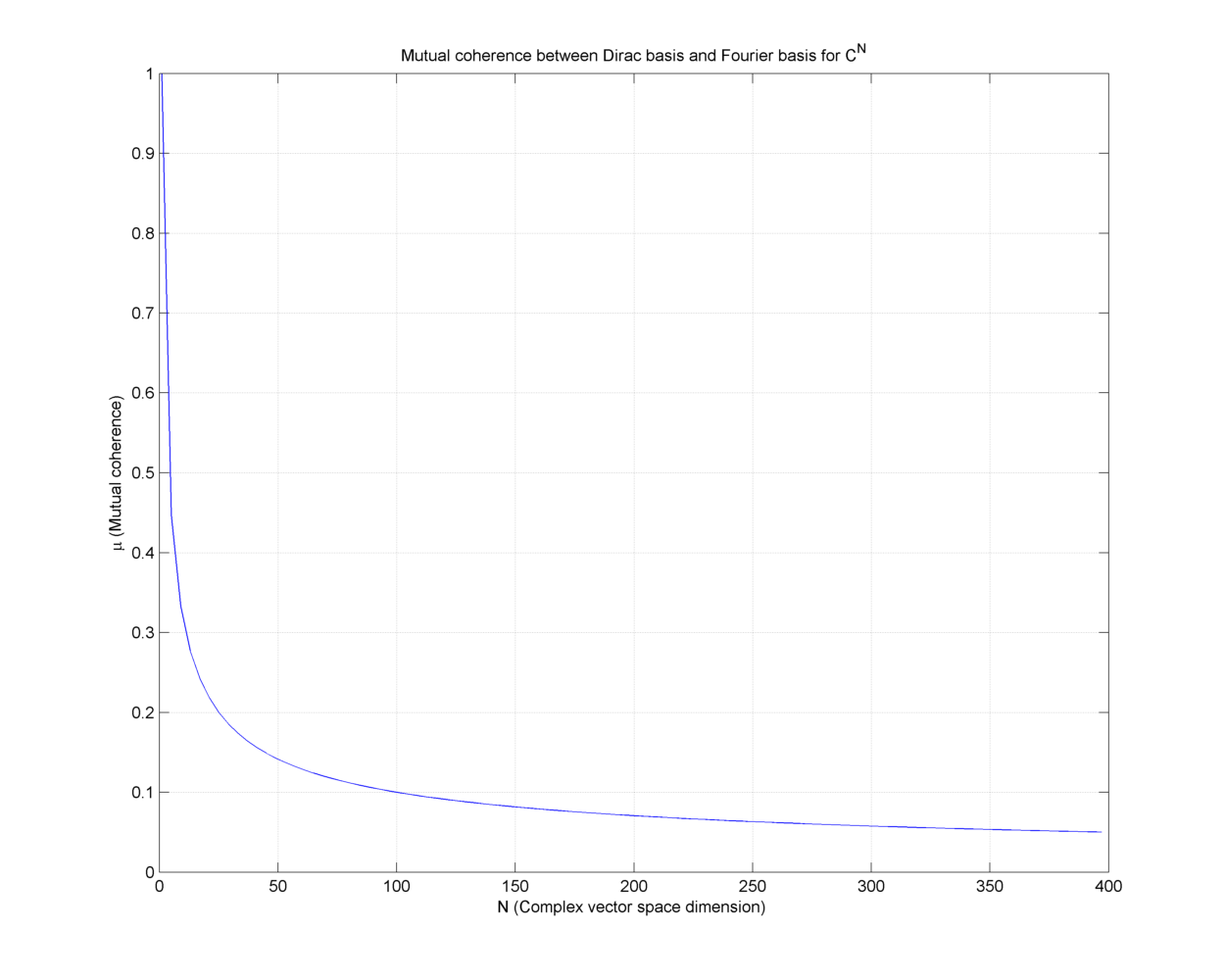
Fig. 18.4 Mutual coherence for Dirac and Fourier bases

We present some results related to mutual coherence of two orthonormal bases.

Theorem 18.2 (Product of orthonormal bases)

The product of two orthonormal bases $\mathrm{\Psi }$ and $\mathcal{X}$ for ${\mathbb{C}}^N$ given by ${\mathrm{\Psi }}^H\mathcal{X}$ forms an orthonormal basis by itself.

Proof. Consider the matrix ${\mathrm{\Psi }}^H\mathcal{X}$

$$\begin{array}{r}{\mathrm{\Psi }}^H\mathcal{X}=\left[\begin{array}{c}{\psi }_1^H\\ \dots \\ {\psi }_N^H\end{array}\right]\left[\begin{array}{ccc}{\chi }_1& \dots & {\chi }_N\end{array}\right]=\left[\begin{array}{cccc}{\psi }_1^H{\chi }_1& {\psi }_1^H{\chi }_2& \dots & {\psi }_1^H{\chi }_N\\ {\psi }_2^H{\chi }_1& {\psi }_2^H{\chi }_2& \dots & {\psi }_2^H{\chi }_N\\ ⋮& ⋮& \ddots & ⋮\\ {\psi }_N^H{\chi }_1& {\psi }_N^H{\chi }_2& \dots & {\psi }_N^H{\chi }_N\end{array}\right]\end{array}$$

Any column of the product matrix is

$$\begin{array}{r}\left[\begin{array}{c}{\psi }_1^H{\chi }_i\\ {\psi }_2^H{\chi }_i\\ ⋮& ⋮\\ {\psi }_N^H{\chi }_i\end{array}\right]={\mathrm{\Psi }}^H{\chi }_i\end{array}$$

But then $\mathrm{\Psi }$ preserves norms, hence

$$\Vert {\mathrm{\Psi }}^H{\chi }_i{\Vert }_2=\Vert {\chi }_i{\Vert }_2=1.$$

Thus each column of the product ${\mathrm{\Psi }}^H\mathcal{X}$ is itself a unit norm vector.

Consider the inner product of two columns of ${\mathrm{\Psi }}^H\mathcal{X}$

$$⟨{\mathrm{\Psi }}^H{\chi }_i,{\mathrm{\Psi }}^H{\chi }_j⟩={\chi }_j^H\mathrm{\Psi }{\mathrm{\Psi }}^H{\chi }_i={\chi }_j^H{\chi }_i=\delta (i-j).$$

Thus, the columns of ${\mathrm{\Psi }}^H\mathcal{X}$ are orthogonal to each other.

Hence ${\mathrm{\Psi }}^H\mathcal{X}$ forms an orthonormal basis.

Remark 18.3 (The group of orthonormal bases)

A more general result would be to show that the set of orthonormal bases forms a group under the matrix multiplication operation. The identity element is the Dirac basis. The inverse of an orthonormal basis is also an orthonormal basis. The product of two orthonormal bases is also an orthonormal basis. The matrix multiplication satisfies associative law.

Theorem 18.3 (Mutual coherence bounds)

Mutual coherence of two orthonormal bases $\mathrm{\Psi }$ and $\mathcal{X}$ for the complex vector space ${\mathbb{C}}^N$ is bounded by

(18.7)$$\frac{1}{\sqrt{N}}\le \mu (\mathrm{\Psi },\mathcal{X})\le 1.$$

Proof. Since columns of both $\mathrm{\Psi }$ and $\mathcal{X}$ are unit norm, hence $|⟨{\psi }_i,{\chi }_j⟩|$ cannot be greater than 1.

Now if $\mathrm{\Psi }=\mathcal{X}$ then we have $\mu (\mathrm{\Psi },\mathcal{X})=1$. This proves the upper bound.

Now consider the matrix ${\mathrm{\Psi }}^H\mathcal{X}$ which forms an orthonormal basis by itself. Consider any column of this matrix

$$\begin{array}{r}\left[\begin{array}{c}{\psi }_1^H{\chi }_i\\ {\psi }_2^H{\chi }_i\\ ⋮& ⋮\\ {\psi }_N^H{\chi }_i\end{array}\right]={\mathrm{\Psi }}^H{\chi }_i\end{array}$$

Since the column is unit norm, hence some of squares of the absolute values of entries of the column is 1. Thus the absolute value of each of the entries cannot be simultaneously less than $\frac{1}{\sqrt{N}}$.

Hence there exists an entry (in each column) such that

$$|{\psi }_j^H{\chi }_i|\ge \frac{1}{\sqrt{N}}.$$

Hence we get the lower bound on mutual coherence of $\mathrm{\Psi }$ and $\mathcal{X}$ given by

$$\mu (\mathrm{\Psi },\mathcal{X})\ge \frac{1}{\sqrt{N}}.$$

Theorem 18.4 (Mutual coherence of Dirac and Fourier bases)

Mutual coherence of Dirac and Fourier bases is $\frac{1}{\sqrt{N}}$.

$$\mu ({\mathbf{I}}_N,{\mathbf{F}}_N)=\frac{1}{\sqrt{N}}.$$

Proof. Theorem 18.3 shows that

$$\mu ({\mathbf{I}}_N,{\mathbf{F}}_N)\ge \frac{1}{\sqrt{N}}.$$

We just need to show that its in fact an equality.

Consider $i$-th column of $\mathbf{I}$ as ${\mathbf{e}}_i$.

Consider $j$-th column of $\mathbf{F}$:

$$\begin{array}{r}{\mathbf{f}}_j=\frac{1}{\sqrt{N}}\left[\begin{array}{c}{\omega }^0\\ {\omega }^j\\ {\omega }^{2j}\\ ⋮\\ {\omega }^{(N-1)j}\end{array}\right]\end{array}$$

where $\omega$ is the $N$-th root of unity. Then

$$⟨{\mathbf{e}}_i,{\mathbf{f}}_j⟩=\frac{1}{\sqrt{N}}{\omega }^{-(i-1)j}⟹|⟨e_i,f_j⟩|=\frac{1}{\sqrt{N}}.$$

This doesn’t depend on the choice of $i$-th column of ${\mathbf{I}}_N$ and $j$-th column of ${\mathbf{F}}_N$. Hence

$$\mu ({\mathbf{I}}_N,{\mathbf{F}}_N)=\frac{1}{\sqrt{N}}.$$

With basic properties of mutual coherence in place, we are now ready to state an uncertainty principle on the sparsity levels of representations of same signal $x$ in two different orthonormal bases:

Theorem 18.5 (Uncertainty principle)

For any arbitrary pair of orthonormal bases $\mathrm{\Psi }$, $\mathcal{X}$ with mutual coherence $\mu (\mathrm{\Psi },\mathcal{X})$, and for any arbitrary non-zero vector $\mathbf{x}\in {\mathbb{C}}^N$ with representations $\mathbf{a}$ and $\mathbf{b}$ respectively, the following inequality holds true:

(18.8)$$\Vert \mathbf{a}{\Vert }_0+\Vert \mathbf{b}{\Vert }_0\ge \frac{2}{\mu (\mathrm{\Psi },\mathcal{X})}.$$

Moreover for unit-length $\mathbf{x}$ we have:

(18.9)$$\Vert \mathbf{a}{\Vert }_1+\Vert \mathbf{b}{\Vert }_1\ge \frac{2}{\sqrt{\mu (\mathrm{\Psi },\mathcal{X})}}.$$

Proof. Dividing $\mathbf{x}$ by $\Vert \mathbf{x}{\Vert }_2$ doesn’t change ${\ell }_0$ “norm” of $\mathbf{a}$ and $\mathbf{b}$. i.e.,

$${\Vert \frac{\mathbf{a}}{\Vert \mathbf{x}{\Vert }_2}\Vert }_0=\Vert \mathbf{a}{\Vert }_0.$$

Hence without loss of generality, we will assume that $\Vert \mathbf{x}{\Vert }_2=1$.

We are given that ${\mathbf{x}}^H\mathbf{x}=1$, $\mathbf{x}=\mathrm{\Psi }\mathbf{a}$ and $\mathbf{x}=\mathcal{X}\mathbf{b}$. Since $\mathrm{\Psi }$ and $\mathcal{X}$ are orthonormal bases hence $\Vert \mathbf{a}{\Vert }_2=\Vert \mathbf{b}{\Vert }_2=1$ also.

We can write

$$\begin{array}{rl}1& ={\mathbf{x}}^H\mathbf{x}\\ & =(\mathrm{\Psi }\mathbf{a}{)}^H(\mathcal{X}\mathbf{b})={\mathbf{a}}^H{\mathrm{\Psi }}^H\mathcal{X}\mathbf{b}\\ & =\sum _{i=1}^N\sum _{j=1}^N\overline{a_i}{b}_j{\psi }_i^H{\chi }_j\\ & =\left|\sum _{i=1}^N\sum _{j=1}^N\overline{a_i}{b}_j{\psi }_i^H{\chi }_j\right|\\ & \le \sum _{i=1}^N\sum _{j=1}^N|a_i||b_j||{\psi }_i^H{\chi }_j|\\ & \le \mu (\mathrm{\Psi },\mathcal{X})\sum _{i=1}^N\sum _{j=1}^N|a_i||b_j|\\ & =\mu (\mathrm{\Psi },\mathcal{X})\Vert \mathbf{a}{\Vert }_1\Vert \mathbf{b}{\Vert }_1\end{array}$$

where we note that

$$\Vert \mathbf{a}{\Vert }_1\Vert \mathbf{b}{\Vert }_1=\left(\sum _{i=1}^N|a_i|\right)\left(\sum _{j=1}^N|b_j|\right)=\sum _{i=1}^N\sum _{j=1}^N|a_i||b_j|$$

and

$$\mu (\mathrm{\Psi },\mathcal{X})\ge |{\psi }_i^H{\chi }_j|.$$

Hence we get the inequality

$$\mu (\mathrm{\Psi },\mathcal{X})\Vert \mathbf{a}{\Vert }_1\Vert \mathbf{b}{\Vert }_1\ge 1$$

Using the inequality between algebraic mean and geometric mean

$$\sqrt{ab}\le \frac{a+b}{2}\mathrm{\forall }a,b\ge 0$$

we get

$$\Vert \mathbf{a}{\Vert }_1+\Vert \mathbf{b}{\Vert }_1\ge 2\sqrt{\Vert \mathbf{a}{\Vert }_1\Vert \mathbf{b}{\Vert }_1}\ge \frac{2}{\sqrt{\mu (\mathrm{\Psi },\mathcal{X})}}.$$

This is an uncertainty principle for the ${\ell }_1$ norms of the two representations. We still have to get the uncertainty principle for ${\ell }_0$ case. Let

$$\Vert \mathbf{a}{\Vert }_0=A\text{ and }\Vert \mathbf{b}{\Vert }_0=B$$

Consider the sets

$$X_A=\{\mathbf{y}|\mathbf{y}=\mathrm{\Psi }\mathbf{u}\text{ and }\Vert \mathbf{u}{\Vert }_0=A,\Vert \mathbf{u}{\Vert }_2=1\}$$

and

$$X_B=\{\mathbf{y}:\mathbf{y}=\mathcal{X}\mathbf{v}\text{ and }\Vert \mathbf{v}{\Vert }_0=B,\Vert \mathbf{v}{\Vert }_2=1\}.$$

Clearly

$$\mathbf{x}\in X_A\cap X_B.$$

The representations $\mathbf{u}$ for vectors $\mathbf{y}$ in $X_A$ have exactly $A$ non-zero entries and are all unit norm representations. Which of them would have the longest ${\ell }_1$ norm $\Vert \mathbf{u}{\Vert }_1$?

This can be written as an optimization problem of the form

(18.10)$$\underset{\mathbf{y}\in X_A}{\text{maximize}}\Vert \mathbf{u}{\Vert }_1\text{ where }\mathbf{u}={\mathrm{\Psi }}^H\mathbf{y}.$$

Let the optimal solution for this problem be ${\mathbf{v}}_a$ with corresponding representation ${\mathbf{a}}^{\ast }={\mathrm{\Psi }}^H{\mathbf{v}}_a$. Clearly

$$\Vert {\mathbf{a}}^{\ast }{\Vert }_1\ge \Vert \mathbf{a}{\Vert }_1.$$

Similarly from the set $X_B$ let us find the vector ${\mathbf{v}}_b$ with maximum ${\ell }_1$ norm representation in $\mathcal{X}$

(18.11)$$\underset{\mathbf{y}\in X_B}{\text{maximize}}\Vert \mathbf{v}{\Vert }_1\text{ where }\mathbf{v}={\mathcal{X}}^H\mathbf{y}.$$

Let the optimal solution for this problem be ${\mathbf{v}}_b$ with corresponding representation ${\mathbf{b}}^{\ast }={\mathcal{X}}^H{\mathbf{v}}_b$. Clearly

$$\Vert {\mathbf{b}}^{\ast }{\Vert }_1\ge \Vert \mathbf{b}{\Vert }_1.$$

Returning back to the inequality

$$\Vert \mathbf{a}{\Vert }_1\Vert \mathbf{b}{\Vert }_1\ge \frac{1}{\mu (\mathrm{\Psi },\mathcal{X})}$$

we can write

$$\Vert {\mathbf{a}}^{\ast }{\Vert }_1\Vert {\mathbf{b}}^{\ast }{\Vert }_1\ge \frac{1}{\mu (\mathrm{\Psi },\mathcal{X})}.$$

An equivalent formulation of the optimization problem (18.10)is

(18.12)$$\begin{array}{rlrl}& \underset{a}{\text{maximize}}& & \Vert \mathbf{a}{\Vert }_1\\ & \text{subject to }& & \Vert \mathbf{a}{\Vert }_2^2={\mathbf{a}}^H\mathbf{a}=1\\ & \text{and }& & \Vert \mathbf{a}{\Vert }_0=A.\end{array}$$

This formulation doesn’t require any specific mention of the basis $\mathrm{\Psi }$. Let the optimal value for this problem be given by

$$\Vert {\mathbf{a}}^{\ast }{\Vert }_1=g(A)=g(\Vert \mathbf{a}{\Vert }_0)$$

Here we consider the optimization problem to be parameterized by the ${\ell }_0$-“norm” of $\mathbf{a}$; i.e., $\Vert \mathbf{a}{\Vert }_0=A$ and we write the optimal value as a function $g$ of the parameter $A$.

Then by symmetry, optimal value for the problem (18.11) is

$$\Vert {\mathbf{b}}^{\ast }{\Vert }_1=g(B)=g(\Vert \mathbf{b}{\Vert }_0)$$

Thus we can write

(18.13)$$g(\Vert \mathbf{a}{\Vert }_0)g(\Vert \mathbf{b}{\Vert }_0)\ge \frac{1}{\mu (\mathrm{\Psi },\mathcal{X})}.$$

This is our intended result since we have been able to write the inequality as a function of ${\ell }_0$ “norm”s of the representations $\mathbf{a}$ and $\mathbf{b}$.

In order to complete the result, we need to find the solution of the optimization problem (18.12) given by the function $g$.

Without loss of generality, let us assume that the $A$ non-zero entries in the optimization variable $\mathbf{a}$ appear in its first $A$ entries and rest are zero. This is fine since changing the order of entries in $\mathbf{a}$ doesn’t affect any of the norms of concern $\Vert \mathbf{a}{\Vert }_0$, $\Vert \mathbf{a}{\Vert }_1$ and $\Vert \mathbf{a}{\Vert }_2$.

Let us further assume that all non-zero entries of $\mathbf{a}$ are strictly positive real numbers. This assumption is valid since only absolute values are used in this problem. Specifically for any $\mathbf{a}$ with non-zero complex entries $(a_1,a_2,\dots ,a_A,0,\dots ,0)$ there exists ${\mathbf{a}}^{\prime }$ with positive entries $(|a_1|,|a_2|,\dots ,|a_A|,0,\dots ,0)$ such that $\Vert \mathbf{a}{\Vert }_0=\Vert {\mathbf{a}}^{\prime }{\Vert }_0$, $\Vert \mathbf{a}{\Vert }_1=\Vert {\mathbf{a}}^{\prime }{\Vert }_1$ and $\Vert \mathbf{a}{\Vert }_2=\Vert {\mathbf{a}}^{\prime }{\Vert }_2$, hence solving the optimization problem for complex $\mathbf{a}$ is same as solving the optimization problem for $\mathbf{a}$ with strictly positive first $A$ entries.

Using Lagrange multipliers, the ${\ell }_0$ constraint vanishes (since the assumptions mentioned above allow us to focus on only the first $A$ coordinates of $\mathbf{a}$), and we obtain

$$\mathcal{L}(\mathbf{a})=\sum _{i=1}^A{a}_i+\lambda (1-\sum _{i=1}^A{a}_i^2).$$

Differentiating w.r.t. $a_i$ and equating to 0 we get

$$1-2\lambda a_i=0⟹a_i=\frac{1}{2\lambda }.$$

The ${\ell }_2$ constraint requires

$$\sum _{i=1}^A{a}_i^2=A\frac{1}{4{\lambda }^2}=1⟹\lambda =\frac{\sqrt{A}}{2}$$

Thus

$$a_i=\frac{1}{\sqrt{A}}$$

and

$$\Vert \mathbf{a}{\Vert }_1=\sum _{i=1}^A|a_i|=\sqrt{A}.$$

Thus the optimal value of the optimization problem (18.12) is

$$g(A)=\sqrt{A}=\sqrt{\Vert \mathbf{a}{\Vert }_0}.$$

Similarly

$$g(B)=\sqrt{B}=\sqrt{\Vert \mathbf{b}{\Vert }_0}.$$

Putting back in (18.13) we get

$$\sqrt{\Vert \mathbf{a}{\Vert }_0\Vert \mathbf{b}{\Vert }_0}\ge \frac{1}{\mu (\mathrm{\Psi },\mathcal{X})}.$$

Applying the algebraic mean-geometric mean inequality we get the desired result

$$\Vert \mathbf{a}{\Vert }_0+\Vert \mathbf{b}{\Vert }_0\ge \frac{2}{\mu (\mathrm{\Psi },\mathcal{X})}.$$

This theorem suggests that if two orthonormal bases have low mutual coherence then

• the two representations for $\mathbf{x}$ cannot be jointly $l_1$-short and

• the two representations for $\mathbf{x}$ cannot be jointly sparse.

Challenge

Can we show that the above result is sharp? i.e. For a pair of orthonormal bases $\mathrm{\Psi }$ and $\mathcal{X}$, it is always possible to find a non-zero vector $\mathbf{x}$ with corresponding representations $\mathbf{x}=\mathrm{\Psi }\mathbf{a}$ and $\mathbf{x}=\mathcal{X}\mathbf{b}$ which satisfies the lower bound

$$\Vert \mathbf{a}{\Vert }_0+\Vert \mathbf{b}{\Vert }_0=\frac{2}{\mu (\mathrm{\Psi },\mathcal{X})}?$$

Example 18.13 (Sparse representations with Dirac and Fourier bases)

We showed in Theorem 18.4 that

$$\mu (\mathbf{I},\mathbf{F})=\frac{1}{\sqrt{N}}.$$

Let $\mathbf{x}\in {\mathbb{C}}^N$. Let its representation in $\mathbf{F}$ be given by

$$\mathbf{x}=\mathbf{F}\mathbf{a}.$$

Applying Theorem 18.5 we have

$$\Vert \mathbf{x}{\Vert }_0+\Vert \mathbf{a}{\Vert }_0\ge \frac{2}{\mu (\mathrm{\Psi },\mathcal{X})}=2\sqrt{N}.$$

This tells us that a signal cannot have fewer than $2\sqrt{N}$ non-zeros in time and frequency domain together.

18.4.4. Linear Combinations of Impulses and Sinusoids

What happens if a signal $\mathbf{x}$ is a linear combination of few complex sinusoids and few impulses?

The set of sinusoids and impulses involved in the construction of $\mathbf{x}$ actually specifies the degrees of freedom of $\mathbf{x}$. This is the indicator of inherent sparsity of $\mathbf{x}$ provided this set of component signals of $\mathbf{x}$ is known a priori.

In absence of prior knowledge of component signals of $\mathbf{x}$, we attempt to look for a sparse representation of $\mathbf{x}$ in one of the well understood orthonormal bases. Here we are specifically looking at the two bases Dirac and Fourier.

While the Dirac basis can provide sparse representation for impulses, sinusoids have dense representation in Dirac basis. Vice versa, in Fourier basis, complex sinusoids have sparse representation, yet impulses have dense representations. Thus neither of the two bases is capable of providing a sparse representation for a combination of impulses and sinusoids.

The natural question arises if there is a way to come up with a sparse representation for such signals by combining the Dirac and Fourier basis?

18.4.5. Dirac Fourier Basis

Now we develop a representation of signals $\mathbf{x}\in {\mathbb{C}}^N$ in terms of a combination of Dirac basis $\mathbf{I}$ and Fourier basis $\mathbf{F}$.

We define a new synthesis matrix

(18.14)$$\mathbf{H}=\left[\begin{array}{cc}\mathbf{I}& \mathbf{F}\end{array}\right]\in {\mathbb{C}}^{N\times 2N}.$$

We can write $\mathbf{I}$ as

$$\mathbf{I}=\left[\begin{array}{ccc}{\mathbf{e}}_1& \dots & {\mathbf{e}}_N\end{array}\right]$$

and $\mathbf{F}$ as

$$\mathbf{F}=\left[\begin{array}{ccc}{\mathbf{f}}_1& \dots & {\mathbf{f}}_N\end{array}\right].$$

This enables us to write $\mathbf{H}$ as

$$\mathbf{H}=\left[\begin{array}{cccccc}{\mathbf{e}}_1& \dots & {\mathbf{e}}_N& {\mathbf{f}}_1& \dots & {\mathbf{f}}_N\end{array}\right].$$

We will look for a representation of $\mathbf{x}$ using the synthesis matrix $\mathbf{H}$ as

$$\mathbf{x}=\mathbf{H}\mathbf{a}$$

where $\mathbf{a}\in {\mathbb{C}}^{2N}$.

Since this representation is under-determined and $\mathcal{C}(\mathbf{H})={\mathbb{C}}^N$ hence there are always infinitely many possible representations of $\mathbf{x}$ in $\mathbf{H}$.

We would prefer to choose the sparsest representation which can be stated as an optimization problem

(18.15)$$\begin{array}{rlrl}& \underset{\mathbf{a}}{\text{minimize}}& & \Vert \mathbf{a}{\Vert }_0\\ & \text{subject to }& & \mathbf{x}=\mathbf{H}\mathbf{a}.\end{array}$$

Example 18.14 (Sparse representation using Dirac Fourier Basis)

Let $N=4$. Then the Dirac Fourier basis is

$$\begin{array}{r}\mathbf{H}=\left[\begin{array}{cccccccc}1& 0& 0& 0& .5& .5& .5& .5\\ 0& 1& 0& 0& .5& .5i& -.5& -.5i\\ 0& 0& 1& 0& .5& -.5& .5& -.5\\ 0& 0& 0& 1& .5& -.5i& -.5& .5i\end{array}\right]\end{array}$$

Let

$$\mathbf{x}=3{\mathbf{e}}_1-2{\mathbf{f}}_2=\left(\begin{array}{cccc}2& -i& 1& i\end{array}\right).$$

A sparse representation of $\mathbf{x}$ in $\mathbf{H}$ is

$$\mathbf{a}=\left(\begin{array}{cccccccc}3& 0& 0& 0& 0& -2& 0& 0\end{array}\right).$$

This representation is $2$-sparse.

Thus we see that Dirac Fourier basis is able to provide a sparser representation of a linear combination of impulses and sinusoids compared to individual orthonormal bases (the Dirac basis and the Fourier basis).

This gives us motivation to consider such combination of bases which help us provide a sparse representation to a larger class of signals. This is the objective of the next section.

In due course we will revisit the Dirac Fourier basis further in several examples.

18.4.6. Two-Ortho Basis

Before we leave this section, let us define general two-ortho bases.

Definition 18.2 (Two ortho basis)

Let $\mathrm{\Psi }$ and $\mathcal{X}$ be any two ${\mathbb{C}}^{N\times N}$ matrices whose columns vectors form orthonormal bases for the complex vector space ${\mathbb{C}}^N$ individually.

We define

(18.16)$$\mathcal{H}=\left[\begin{array}{cc}\mathrm{\Psi }& \mathcal{X}\end{array}\right]\in {\mathbb{C}}^{N\times 2N}.$$

The columns of $\mathcal{H}$ form a two-ortho basis for ${\mathbb{C}}^N$.

Clearly columns of $\mathcal{H}$ span ${\mathbb{C}}^N$.

Remark 18.4 (Coherence of a two ortho basis)

The coherence of a two ortho basis is defined as

$$\mu (\mathcal{H})=\mu (\mathrm{\Psi },\mathcal{X}).$$

It is the magnitude of the largest inner product between columns of $\mathcal{H}$.

We present a very interesting result about the null space of $\mathcal{H}$.

Theorem 18.6 (Denseness of vectors in null space of two ortho bases)

For a two ortho basis $\mathcal{H}=\left[\begin{array}{cc}\mathrm{\Psi }& \mathcal{X}\end{array}\right]$ with low coherence, the non-zero vectors in the null space of $\mathcal{H}$ are not sparse.

Concretely

$$\Vert \mathbf{v}{\Vert }_0\ge \frac{2}{\mu (\mathcal{H})}\mathrm{\forall }\mathbf{v}\in \mathcal{N}(\mathcal{H}).$$

Proof. Let $\mathbf{v}\in \mathcal{N}(\mathcal{H})$ be some non-zero vector.

Now let ${\mathbf{v}}_{\psi }$ and ${\mathbf{v}}_{\chi }$ be first N and last N entries of $\mathbf{v}$. Then

$$\begin{array}{r}\left[\begin{array}{cc}\mathrm{\Psi }& \mathcal{X}\end{array}\right]\left[\begin{array}{c}{\mathbf{v}}_{\psi }\\ {\mathbf{v}}_{\chi }\end{array}\right]=\mathbf{0}⟹\mathrm{\Psi }{\mathbf{v}}_{\psi }=-\mathcal{X}{\mathbf{v}}_{\chi }=\mathbf{y}\ne \mathbf{0}.\end{array}$$

If $\mathbf{y}$ were $\mathbf{0}$, then both ${\mathbf{v}}_{\psi }$ and ${\mathbf{v}}_{\chi }$ would have to be $\mathbf{0}$ which is not the case since by assumption $\mathbf{v}\ne \mathbf{0}$.

We note that ${\mathbf{v}}_{\psi }$ and $-{\mathbf{v}}_{\chi }$ are representations of same vector $\mathbf{y}$ in two different orthonormal bases $\mathrm{\Psi }$ and $\mathcal{X}$ respectively, and $\Vert -{\mathbf{v}}_{\chi }{\Vert }_0=\Vert {\mathbf{v}}_{\chi }{\Vert }_0$.

Applying Theorem 18.5 we have

$$\Vert \mathbf{v}{\Vert }_0=\Vert {\mathbf{v}}_{\psi }{\Vert }_0+\Vert {\mathbf{v}}_{\chi }{\Vert }_0\ge \frac{2}{\mu (\mathcal{H})}.$$

We also note that since the orthonormal bases preserve norm, hence

$$\Vert \mathbf{y}{\Vert }_2=\Vert {\mathbf{v}}_{\psi }{\Vert }_2=\Vert {\mathbf{v}}_{\chi }{\Vert }_2.$$

This shows us that the energy of a null space vector is evenly distributed in the two components corresponding to each orthonormal basis.

Challenge

For a two-ortho basis $\mathcal{H}=\left[\begin{array}{cc}\mathrm{\Psi }& \mathcal{X}\end{array}\right]$ is it possible to find a null space vector $\mathbf{v}$ satisfying the lower bound

$$\Vert \mathbf{v}{\Vert }_0=\frac{2}{\mu (\mathcal{H})}?$$

Let $\mathbf{x}\in {\mathbb{C}}^N$ be any arbitrary signal. Then its representation in $\mathcal{H}$ is given by

$$\mathbf{x}=\mathcal{H}\mathbf{a}.$$

Obviously for every $\mathbf{z}\in \mathcal{N}(\mathcal{H})$, the vector $\mathbf{a}+\mathbf{z}$ is also a representation of $\mathbf{x}$.

What we are particularly interested in are sparse representations of $\mathbf{x}$. A key concern for us is to ensure that a sparse representation of $\mathbf{x}$ in $\mathcal{H}$ is unique. Under what conditions such is possible?

Formally, let $\mathbf{a}$ and $\mathbf{b}$ be two different representations of $\mathbf{x}$ in $\mathcal{H}$. Can we say that if $\mathbf{a}$ is sparse then $\mathbf{b}$ won’t be sparse?

This is established in the next uncertainty principle.

Theorem 18.7 (Uncertainty principle for representations in two ortho basis)

Let $\mathbf{x}\in {\mathbb{C}}^N$ be any signal and let $\mathcal{H}$ be a two ortho basis defined in (18.16). Let $\mathbf{a}$ and $\mathbf{b}$ be two distinct representations of $\mathbf{x}$ in $\mathcal{H}$ i.e.

$$\mathbf{x}=\mathcal{H}\mathbf{a}=\mathcal{H}\mathbf{b}.$$

Then the following holds

$$\Vert \mathbf{a}{\Vert }_0+\Vert \mathbf{b}{\Vert }_0\ge \frac{2}{\mu (\mathcal{H})}.$$

This is an uncertainty principle for the sparsity of distinct representations in two ortho basis.

Proof. Let

$$\mathbf{e}=\mathbf{a}-\mathbf{b}$$

be the difference vector of representations of $\mathbf{x}$. Clearly

$$\mathcal{H}\mathbf{e}=\mathcal{H}\mathbf{a}-\mathcal{H}\mathbf{b}=\mathbf{x}-\mathbf{x}=\mathbf{0}.$$

Thus $\mathbf{e}\in \mathcal{N}(\mathcal{H})$. Applying Theorem 18.6, we get

$$\Vert \mathbf{e}{\Vert }_0\ge \frac{2}{\mu (\mathcal{H})}.$$

But since $\mathbf{e}=\mathbf{a}-\mathbf{b}$ hence we have

$$\Vert \mathbf{a}{\Vert }_0+\Vert \mathbf{b}{\Vert }_0\ge \Vert \mathbf{e}{\Vert }_0\ge \frac{2}{\mu (\mathcal{H})}.$$

Challenge

For a two-ortho basis $\mathcal{H}=\left[\begin{array}{cc}\mathrm{\Psi }& \mathcal{X}\end{array}\right]$ is it possible to find a vector $\mathbf{x}$ with two alternative representations $\mathbf{a}$ and $\mathbf{b}$ satisfying the lower bound

$$\Vert \mathbf{a}{\Vert }_0+\Vert \mathbf{b}{\Vert }_0=\frac{2}{\mu (\mathcal{H})}?$$

This theorem suggests as that if $\mu (\mathcal{H})$ is small (i.e. the coherence between the two orthonormal bases is small) then two representations of $\mathbf{x}$ cannot be simultaneously sparse.

Rather if a representation is sufficiently sparse, then all other representations of $\mathbf{x}$ are guaranteed to be non-sparse providing the uniqueness of sparse representation.

This is stated formally in the following uniqueness theorem.

Theorem 18.8 (Uniqueness of sparse representation in two ortho basis)

If a representation of $\mathbf{x}$ in the two ortho basis $\mathcal{H}=\left[\begin{array}{cc}\mathrm{\Psi }& \mathcal{X}\end{array}\right]$ has fewer than $\frac{1}{\mu (\mathcal{H})}$ non-zero entries, then it is necessarily the sparsest one possible, and any other representation must be denser.

Proof. Let $\mathbf{a}$ be a candidate representation with

$$\Vert \mathbf{a}{\Vert }_0<\frac{1}{\mu (\mathcal{H})}.$$

Let $\mathbf{b}$ be any other candidate representation. By applying Theorem 18.7 we have

$$\Vert \mathbf{a}{\Vert }_0+\Vert \mathbf{b}{\Vert }_0\ge \frac{2}{\mu (\mathcal{H})}.$$

This gives us

$$\Vert \mathbf{b}{\Vert }_0\ge \frac{2}{\mu (\mathcal{H})}-\Vert \mathbf{a}{\Vert }_0⟹\Vert \mathbf{b}{\Vert }_0>\frac{1}{\mu (\mathcal{H})}.$$

Thus we find that

$$\Vert \mathbf{b}{\Vert }_0>\Vert \mathbf{a}{\Vert }_0$$

which is true for every representation $\mathbf{b}$ of $\mathbf{x}$ in $\mathcal{H}$ other than $\mathbf{a}$.

Hence $\mathbf{a}$ is the sparsest possible representation of $\mathbf{x}$ in $\mathcal{H}$.

We note here that any arbitrary choice of two bases may not be helpful in coming up with a two ortho basis which can provide us sparse representations for our signals of interest. In next few sections, we will explore this issue further in the more general context of signal dictionaries.

Challenge

Clearly, are signals for which a sufficiently sparse (and unique) representation doesn’t exist in a given two-ortho basis. What kind of relationships may exist between different (insufficiently) sparse representations of such signals?

18.4.7. Dirac-DCT Basis

Dirac Fourier 2-ortho-basis is optimal in the sense that it has the smallest mutual coherence between the two bases. However, one problem with the Dirac Fourier basis is that it requires us to work with complex numbers. A close second is the Dirac DCT basis which consists of the Dirac basis and the DCT basis both of which are real.

Definition 18.3 (Dirac DCT basis)

The Dirac-DCT basis is a two-ortho basis consisting of the union of the Dirac and the DCT bases.

This two ortho basis is suitable for real signals since both Dirac and DCT are totally real bases $\in {\mathbb{R}}^{N\times N}$.

The two ortho basis is obtained by combining the $N\times N$ identity matrix (Dirac basis) with the $N\times N$ DCT matrix for signals in ${\mathbb{R}}^N$.

Let ${\mathrm{\Psi }}_{\text{DCT},N}$ denote the DCT matrix for ${\mathbb{R}}^N$. Let ${\mathbf{I}}_N$ denote the identity matrix for ${\mathbb{R}}^N$. Then

$${\mathcal{D}}_{\text{DCT}}=\left[\begin{array}{cc}{\mathbf{I}}_N& {\mathrm{\Psi }}_{\text{DCT},N}\end{array}\right].$$

Let

$${\mathrm{\Psi }}_{\text{DCT},N}=\left[\begin{array}{cccc}{\psi }_1& {\psi }_2& \dots & {\psi }_N\end{array}\right]$$

The $k$-th column of ${\mathrm{\Psi }}_{\text{DCT},N}$ is given by

(18.17)$${\psi }_k(n)=\sqrt{\frac{2}{N}}{\mathrm{\Omega }}_k\cos (\frac{\pi }{2N}(2n-1)(k-1)),n=1,\dots ,N,$$

with ${\mathrm{\Omega }}_k=\frac{1}{\sqrt{2}}$ for $k=1$ and ${\mathrm{\Omega }}_k=1$ for $2\le k\le N$.

Note that for $k=1$, the entries become

$$\sqrt{\frac{2}{N}}\frac{1}{\sqrt{2}}\cos 0=\sqrt{\frac{1}{N}}.$$

Thus, the ${\ell }_2$ norm of ${\psi }_1$ is 1. We can similarly verify the ${\ell }_2$ norm of other columns also. They are all one.

18.4.7.1. Example

We show how a mixture signal consisting of impulses and sinusoids has a sparse representation in a Dirac DCT basis.

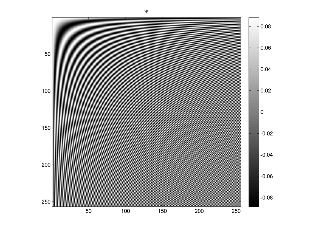
Fig. 18.5 A DCT basis for $N=256$

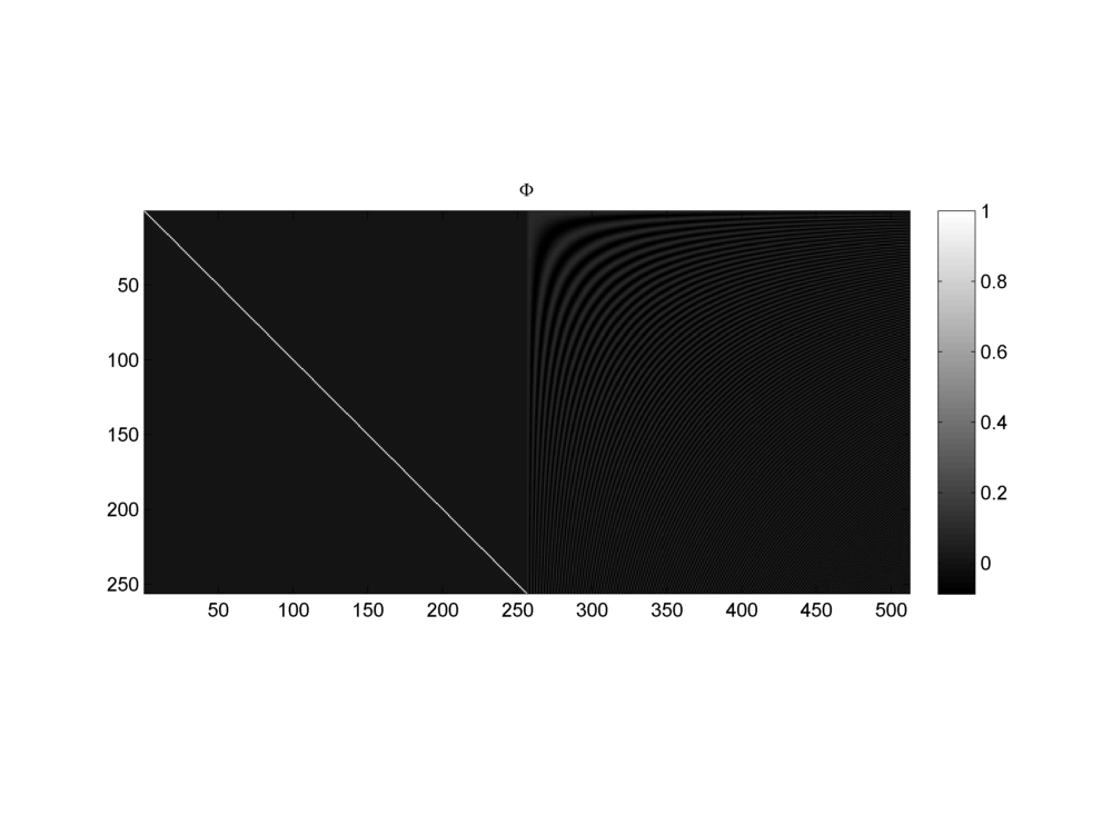
Fig. 18.6 A Dirac DCT basis for $N=256$ and $D=512$.

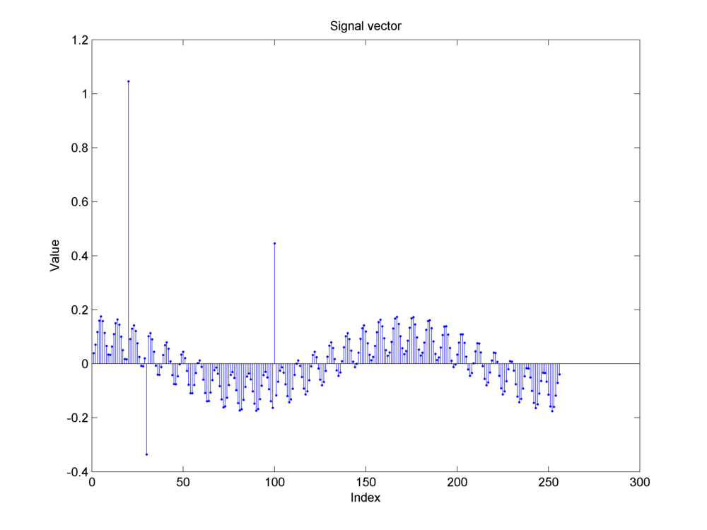
Fig. 18.7 An $N=256$ length signal consisting of a mixture of $3$ impulses and $2$ cosine signals.

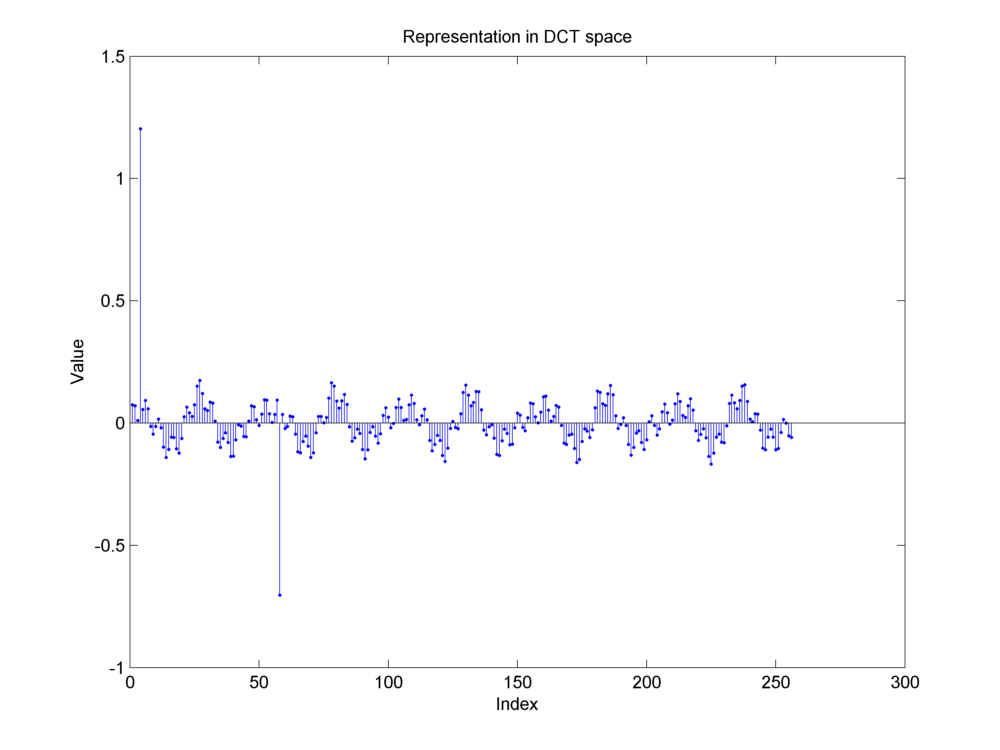
Fig. 18.8 Representation of the same mixture signal in DCT basis. Notice the two large magnitude components. They correspond to the two sinusoidal components in the original time domain signal. The three impulses in the time domain signal have been distributed among all the frequencies.

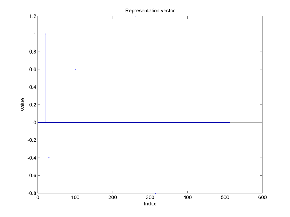
Fig. 18.9 A sparse representation of the same mixture signal in the two ortho Dirac-DCT basis. The three impulses from the original signal appear on the left half (corresponding to the Dirac basis part). The two cosine sinusoids appear on the right half (corresponding to the DCT basis part). Indeed the representation is not unique. But it is the unique sparsest possible representation. All other representations have far more nonzero components.

18.4.7.2. Coherence

Theorem 18.9

The Dirac-DCT basis has the mutual coherence of $\sqrt{\frac{2}{N}}$.

Proof. The mutual coherence of a two ortho basis where one basis is Dirac basis is given by the magnitude of the largest entry in the other basis.

1. For ${\mathrm{\Psi }}_{\text{DCT},N}$, the largest value is obtained when ${\mathrm{\Omega }}_k=1$ and the $\cos$ term evaluates to 1.

2. Clearly,

   $$\mu ({\mathcal{D}}_{\text{DCT}})=\sqrt{\frac{2}{N}}.$$

18.4.7.3. Construction of Sparse Representation

We use sparse recovery/reconstruction algorithms to construct a sparse representation of a given signal in a two ortho basis. The algorithms will be discussed in later chapters. We give the time domain signal (e.g. the mixture signal above) and the two ortho basis to a sparse reconstruction algorithm. The algorithm attempts to construct a sparsest possible representation of the signal in the given two ortho basis. We reconstructed this mixture signal in Dirac DCT basis using three different algorithms:

• Basis Pursuit

• Matching Pursuit

• Orthogonal Matching Pursuit

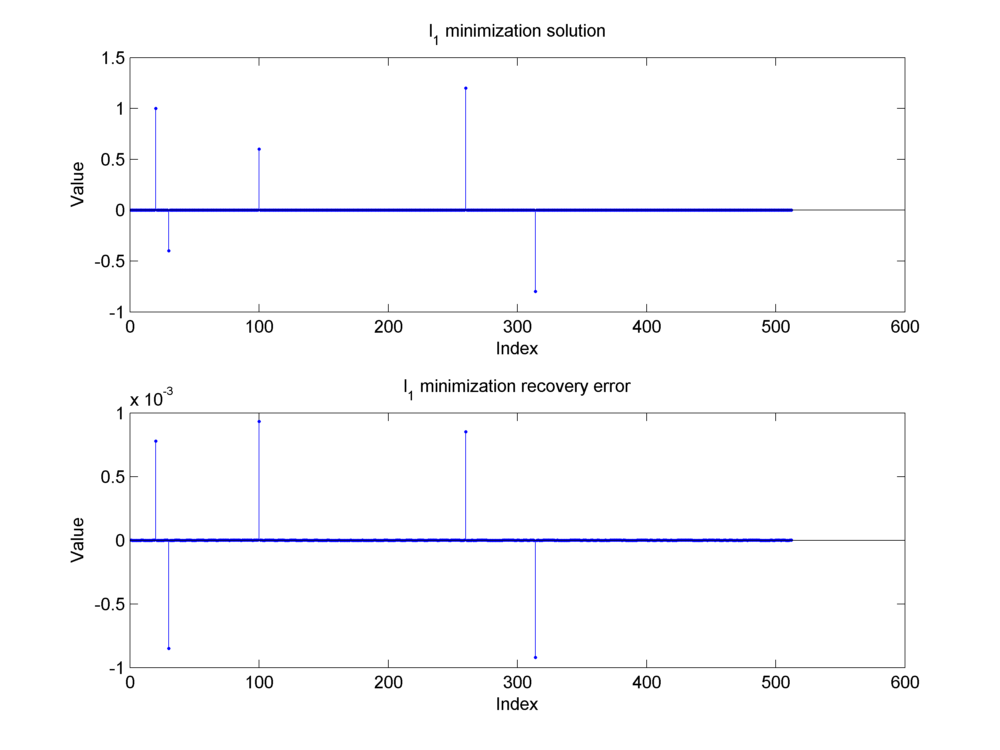
Fig. 18.10 Construction of the sparse representation of the mixture signal using the basis pursuit algorithm.

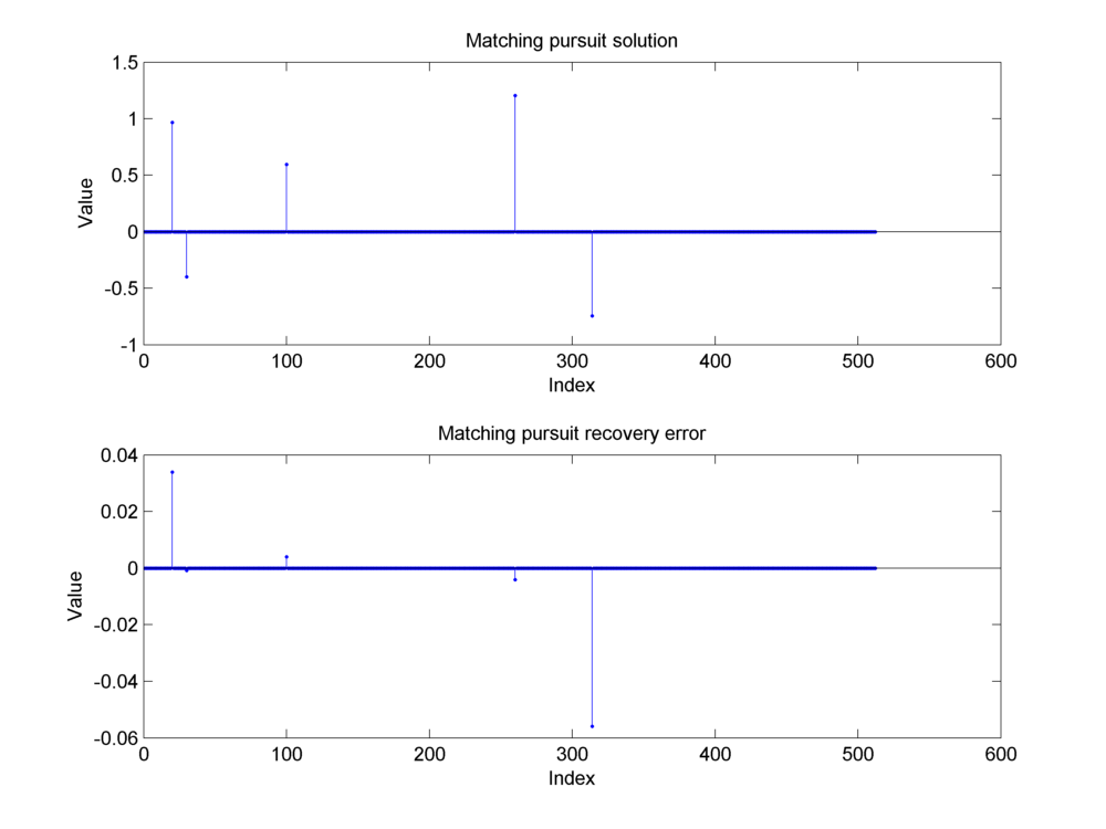
Fig. 18.11 Construction of the sparse representation of the mixture signal using the matching pursuit algorithm.

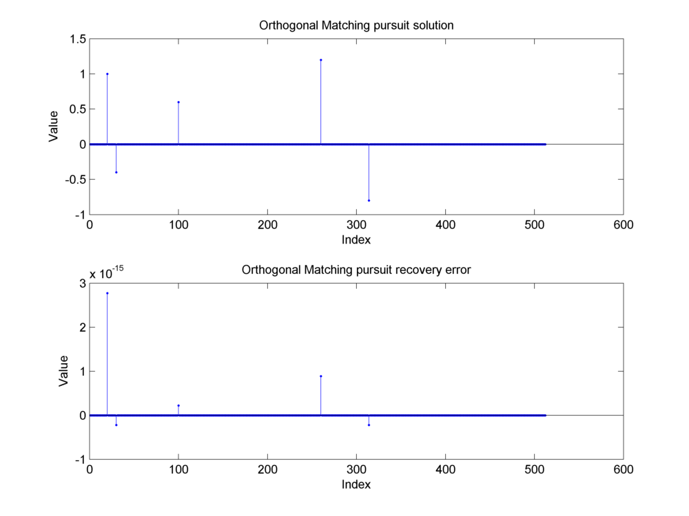
Fig. 18.12 Construction of the sparse representation of the mixture signal using the orthogonal matching pursuit algorithm.